Statistical Methods in AIML Bucket elimination Vibhav Gogate
Statistical Methods in AI/ML Bucket elimination Vibhav Gogate
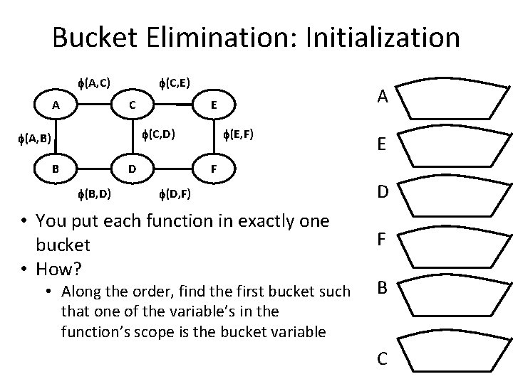
Bucket Elimination: Initialization (A, C) A (C, E) C (C, D) (A, B) B A E D (E, F) E F (D, F) D • You put each function in exactly one bucket • How? F (B, D) • Along the order, find the first bucket such that one of the variable’s in the function’s scope is the bucket variable B C
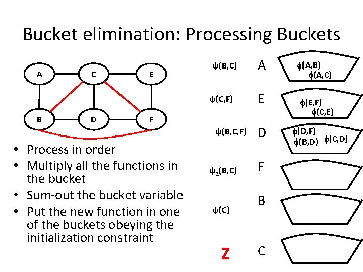
Bucket elimination: Processing Buckets A C E ψ(B, C) ψ(C, F) B D F ψ(B, C, F) • Process in order • Multiply all the functions in the bucket • Sum-out the bucket variable • Put the new function in one of the buckets obeying the initialization constraint ψ2(B, C) ψ(C) Z A E D F B C (A, B) (A, C) (E, F) (C, E) (D, F) (B, D) (C, D)
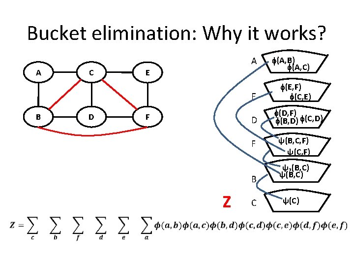
Bucket elimination: Why it works? A C A E E B D F B Z C (A, B) (A, C) (E, F) (C, E) (D, F) (B, D) (C, D) ψ(B, C, F) ψ(C, F) ψ2(B, C) ψ(C)
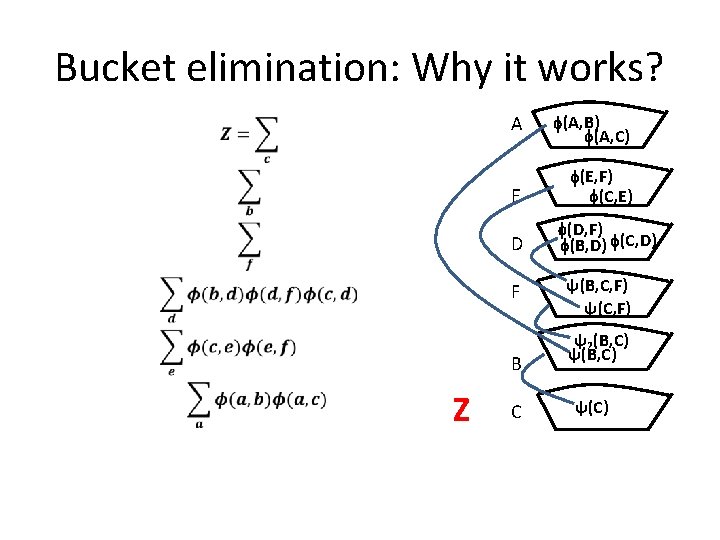
Bucket elimination: Why it works? A E D F B Z C (A, B) (A, C) (E, F) (C, E) (D, F) (B, D) (C, D) ψ(B, C, F) ψ(C, F) ψ2(B, C) ψ(C)
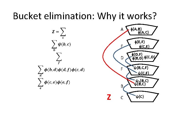
Bucket elimination: Why it works? A E D F B Z C (A, B) (A, C) (E, F) (C, E) (D, F) (B, D) (C, D) ψ(B, C, F) ψ(C, F) ψ2(B, C) ψ(C)
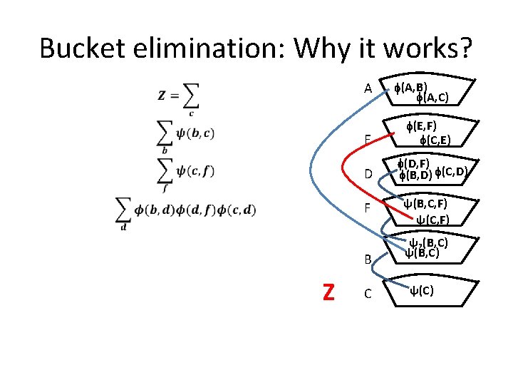
Bucket elimination: Why it works? A E D F B Z C (A, B) (A, C) (E, F) (C, E) (D, F) (B, D) (C, D) ψ(B, C, F) ψ(C, F) ψ2(B, C) ψ(C)
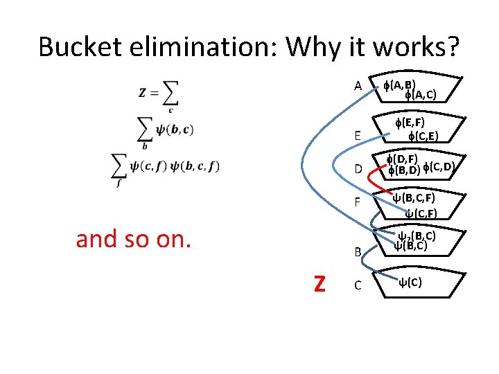
Bucket elimination: Why it works? A E D F and so on. B Z C (A, B) (A, C) (E, F) (C, E) (D, F) (B, D) (C, D) ψ(B, C, F) ψ(C, F) ψ2(B, C) ψ(C)
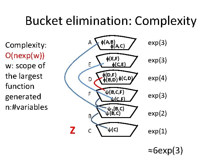
Bucket elimination: Complexity A Complexity: O(nexp(w)) w: scope of the largest function generated n: #variables E D F B Z C (A, B) (A, C) exp(3) (E, F) (C, E) exp(3) (D, F) (B, D) (C, D) exp(4) ψ(B, C, F) ψ(C, F) exp(3) ψ2(B, C) ψ(B, C) exp(2) ψ(C) exp(1) ≈6 exp(3)
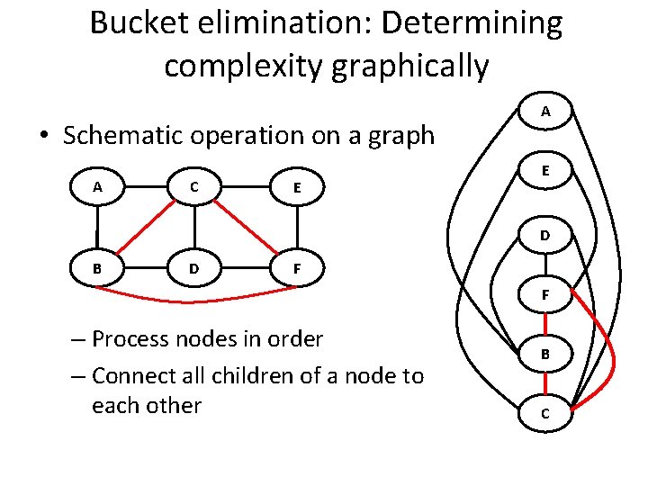
Bucket elimination: Determining complexity graphically • Schematic operation on a graph A C E A E D B D F F – Process nodes in order – Connect all children of a node to each other B C
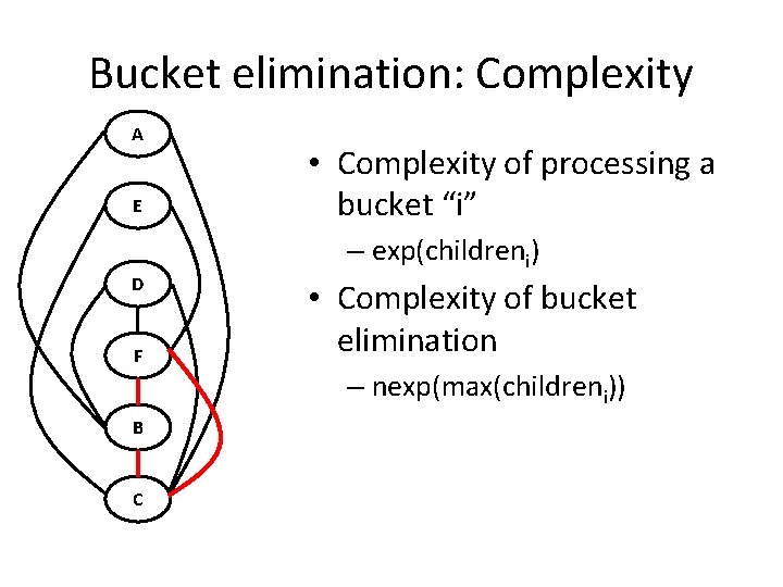
Bucket elimination: Complexity A E D F B C • Complexity of processing a bucket “i” – exp(childreni) • Complexity of bucket elimination – nexp(max(childreni))
Treewidth and Tree Decompositions • Running schematic bucket elimination yields a chordal graph – Each cycle of length > 3 has a chord (an edge connecting two nodes that are not adjacent in the cycle) • Every chordal graph can be represented using a tree decomposition
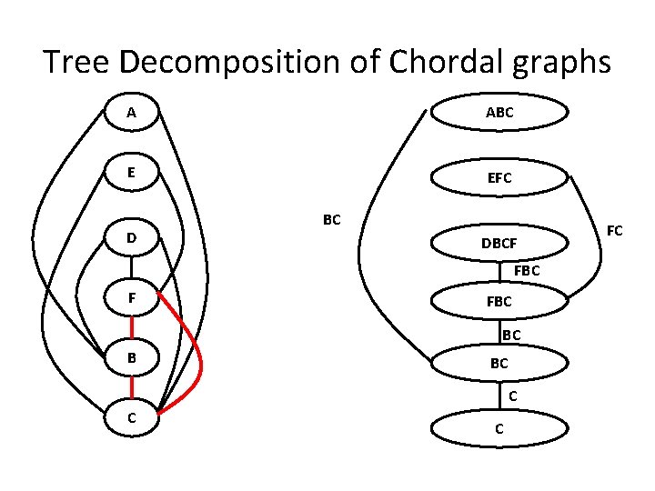
Tree Decomposition of Chordal graphs A ABC E EFC D BC DBCF FBC BC B BC C FC
Tree Decomposition and Treewidth: Definition • Given a network and its interaction graph • Tree Decomposition is a set of subset of variables connected by a tree such that: – Each variable is present in at least one subset – Each edge is present in at least one subset – The set of subsets containing a variable “X” form a connected sub-tree • Running intersection property • Width of a tree decomposition: Cardinality of the maximum subset minus 1 • Treewidth: minimum width out of all possible tree decompositions
Bucket elimination: Complexity • Best possible complexity: O(nexp(w+1)) where w is the treewidth of the graph • Thus, we have a graph-based algorithm for determining the complexity of bucket elimination. • If w is small, we can solve the problem efficiently!
Generating Tree Decompositions • Computing treewidth is NP-hard • Branch and Bound algorithm (Gogate&Dechter, 2004) • Best-first search algorithm – (Dow and Korf, 2009) • Heuristics in practice – min-fill heuristic – min-degree heuristic
Min-degree and min-fill • min-degree – At each point, select a variable with minimum degree (ties broken arbitrarily) – Connect the children of the variable to each other • min-fill – At each point, select a variable that adds the minimum number of edges to the current graph – Connect the children of the selected variable to each other
Computing all Marginals • Bucket elimination computes – P(e) or Z – P(Xi|e) where “Xi” is the last variable eliminated • To compute all marginals P(Xi|e) for all variables Xi – Run bucket elimination “n” times • Efficient algorithm – Junction tree algorithm or bucket tree propagation – Requires only two passes to compute all marginals
Junction tree algorithm: An exact message passing algorithm • Construct a tree decomposition T • Initialize the tree decomposition as in bucket elimination • Select an arbitrary node of T as root • Pass messages from leaves to root (upward pass) • Pass messages from root to leaves (downward pass)
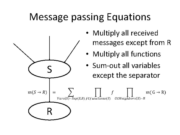
Message passing Equations S R • Multiply all received messages except from R • Multiply all functions • Sum-out all variables except the separator
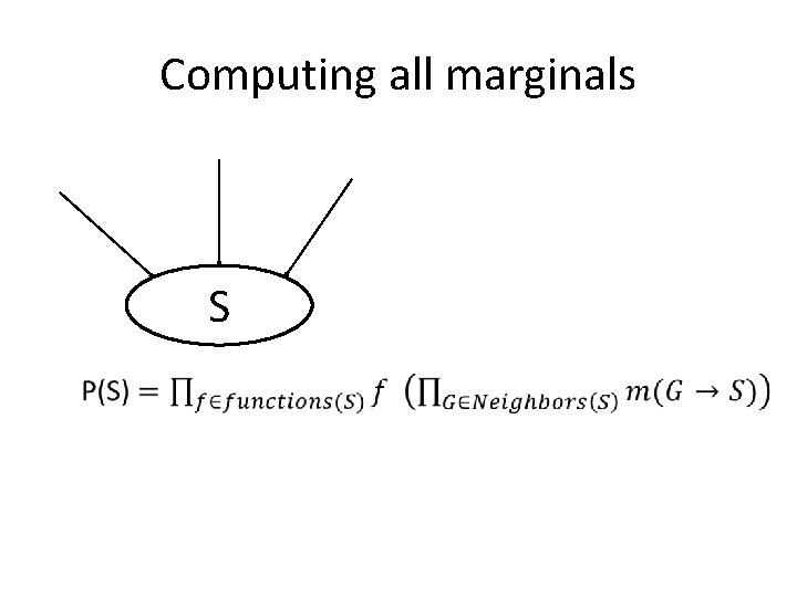
Computing all marginals S
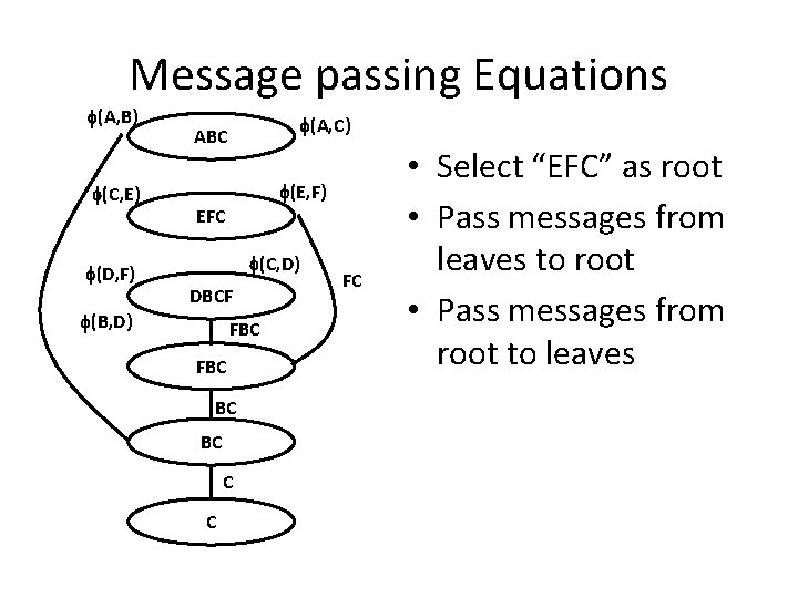
Message passing Equations (A, B) (C, E) (D, F) (A, C) ABC (E, F) EFC (C, D) DBCF (B, D) FBC BC BC C C FC • Select “EFC” as root • Pass messages from leaves to root • Pass messages from root to leaves
Architectures • Shenoy-Shafer architecture • Hugin architecture – Associate one function with each cluster – Requires multiplication – Smaller time complexity – Higher space complexity
- Slides: 23