Statistical Learning Methods Chapter 20 20 1 20

Statistical Learning Methods Chapter 20 (20. 1, 20. 2, 20. 3, 20. 4) Copyright, 1996 © Dale Carnegie & Associates, Inc.

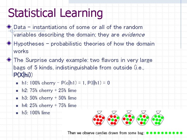
Statistical Learning Data – instantiations of some or all of the random variables describing the domain; they are evidence Hypotheses – probabilistic theories of how the domain works The Surprise candy example: two flavors in very large bags of 5 kinds, indistinguishable from outside (i. e. , P(X|hi)) n n n h 1: h 2: h 3: h 4: h 5: 100% cherry – P(c|h 1) = 1, P(l|h 1) = 0 75% cherry + 25% lime 50% cherry + 50% lime 25% cherry + 75% lime 100% lime CSE 471/598 by H. Liu 2

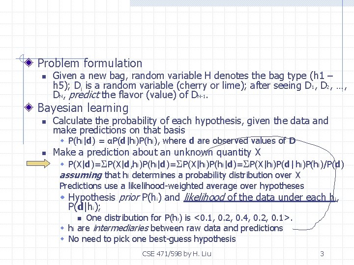
Problem formulation n Given a new bag, random variable H denotes the bag type (h 1 – h 5); Di is a random variable (cherry or lime); after seeing D 1, D 2, …, DN, predict the flavor (value) of DN-1. Bayesian learning n Calculate the probability of each hypothesis, given the data and make predictions on that basis w P(hi|d) = αP(d|hi)P(hi), where d are observed values of D n Make a prediction about an unknown quantity X w P(X|d)= i. P(X|d, hi)P(hi|d)= i. P(X|hi)P(d|hi)P(hi)/P(d) assuming that hi determines a probability distribution over X Predictions use a likelihood-weighted average over hypotheses w Hypothesis prior P(hi) and likelihood of the data under each hi, P(d|hi); One distribution for P(hi) is <0. 1, 0. 2, 0. 4, 0. 2, 0. 1>. w hi are intermediaries between raw data and predictions w No need to pick one best-guess hypothesis n CSE 471/598 by H. Liu 3

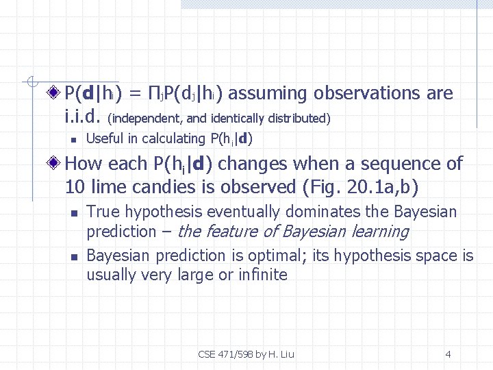
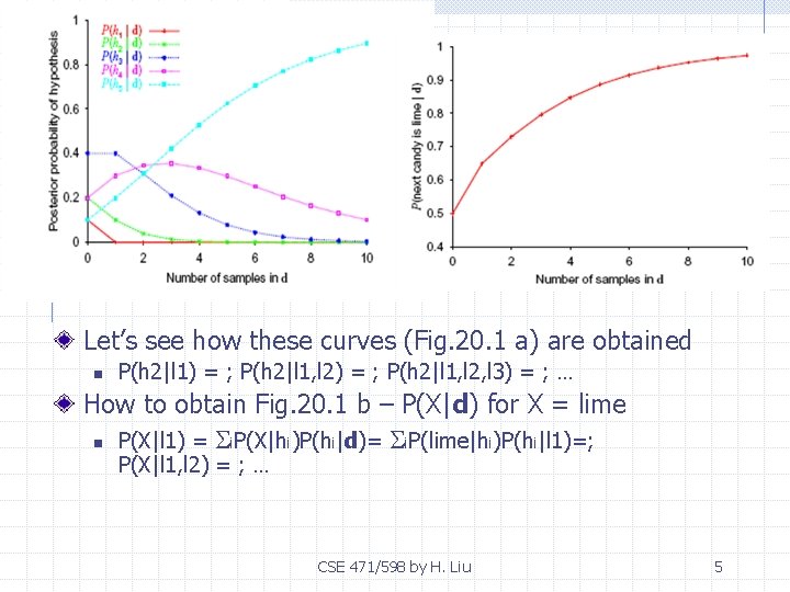
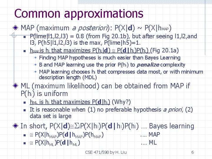
P(d|hi) = Πj. P(dj|hi) assuming observations are i. i. d. (independent, and identically distributed) n Useful in calculating P(hi|d) How each P(hi|d) changes when a sequence of 10 lime candies is observed (Fig. 20. 1 a, b) n n True hypothesis eventually dominates the Bayesian prediction – the feature of Bayesian learning Bayesian prediction is optimal; its hypothesis space is usually very large or infinite CSE 471/598 by H. Liu 4

Let’s see how these curves (Fig. 20. 1 a) are obtained n P(h 2|l 1) = ; P(h 2|l 1, l 2, l 3) = ; … How to obtain Fig. 20. 1 b – P(X|d) for X = lime n P(X|l 1) = i. P(X|hi)P(hi|d)= i. P(lime|hi)P(hi|l 1)=; P(X|l 1, l 2) = ; … CSE 471/598 by H. Liu 5

Common approximations MAP (maximum a posteriori): P(X|d) ~ P(X|h. MAP) n n P(lime|l 1, l 2, l 3) = 0. 8 (from Fig 20. 1 b), but after seeing l 1, l 2, and l 3, P(h 5|l 1, l 2, l 3) is the max, P(lime|h 5)=1. h. MAP is hi that maximizes P(hi|d) P(d|hi)P(hi) (Fig 20. 1 a) w Finding MAP hypotheses is much easier than Bayes Learning w B and MAP learning use the prior P(hi) to penalize complexity w MAP learning chooses hi that compresses data most, or with minimum description length (MDL) ML (maximum likelihood) can be obtained from MAP if P(hi) is uniform n n h. ML is hi that maximizes P(d|hi) (Why? ) It is reasonable when (1) no preferable hypothesis a priori, (2) data set is large In short, P(X|d) i. P(X|hi)P(d|hi)P(hi) … Bayes learning n n P(X|h. MAP)P(d|h. MAP)P(h. MAP) P(X|h. ML)P(d|h. ML) CSE 471/598 by H. Liu . … MAP. … ML 6

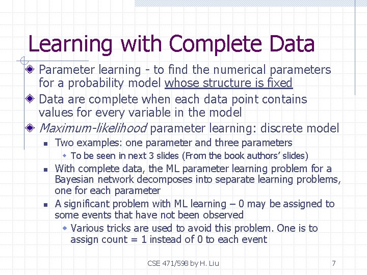
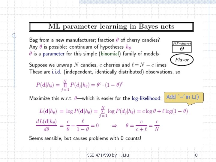
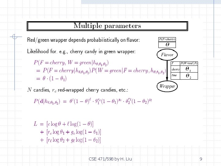
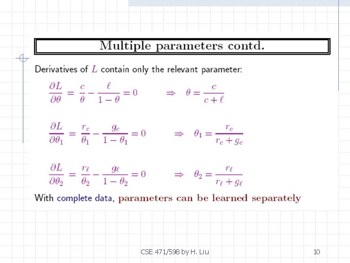
Learning with Complete Data Parameter learning - to find the numerical parameters for a probability model whose structure is fixed Data are complete when each data point contains values for every variable in the model Maximum-likelihood parameter learning: discrete model n Two examples: one parameter and three parameters w To be seen in next 3 slides (From the book authors’ slides) n n With complete data, the ML parameter learning problem for a Bayesian network decomposes into separate learning problems, one for each parameter A significant problem with ML learning – 0 may be assigned to some events that have not been observed w Various tricks are used to avoid this problem. One is to assign count = 1 instead of 0 to each event CSE 471/598 by H. Liu 7

Add `–’ in L() CSE 471/598 by H. Liu 8

CSE 471/598 by H. Liu 9

CSE 471/598 by H. Liu 10

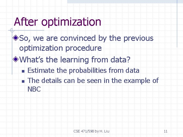
After optimization So, we are convinced by the previous optimization procedure What’s the learning from data? n n Estimate the probabilities from data The details can be seen in the example of NBC CSE 471/598 by H. Liu 11

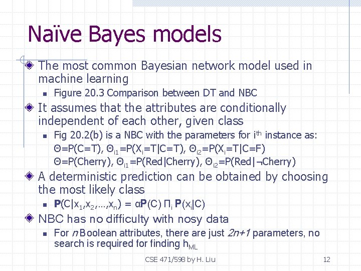
Naïve Bayes models The most common Bayesian network model used in machine learning n Figure 20. 3 Comparison between DT and NBC It assumes that the attributes are conditionally independent of each other, given class n Fig 20. 2(b) is a NBC with the parameters for ith instance as: Θ=P(C=T), Θi 1=P(Xi=T|C=T), Θi 2=P(Xi=T|C=F) Θ=P(Cherry), Θi 1=P(Red|Cherry), Θi 2=P(Red|¬Cherry) A deterministic prediction can be obtained by choosing the most likely class n P(C|x 1, x 2, …, xn) = αP(C) Πi P(xi|C) NBC has no difficulty with nosy data n For n Boolean attributes, there are just 2 n+1 parameters, no search is required for finding h. ML CSE 471/598 by H. Liu 12

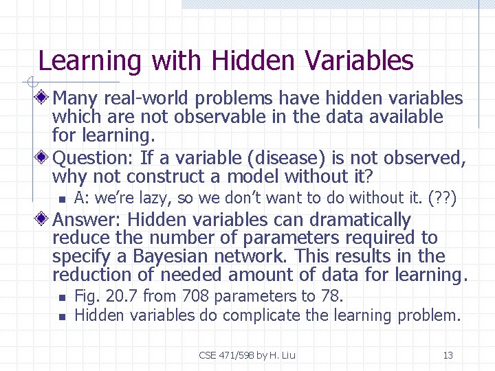
Learning with Hidden Variables Many real-world problems have hidden variables which are not observable in the data available for learning. Question: If a variable (disease) is not observed, why not construct a model without it? n A: we’re lazy, so we don’t want to do without it. (? ? ) Answer: Hidden variables can dramatically reduce the number of parameters required to specify a Bayesian network. This results in the reduction of needed amount of data for learning. n n Fig. 20. 7 from 708 parameters to 78. Hidden variables do complicate the learning problem. CSE 471/598 by H. Liu 13

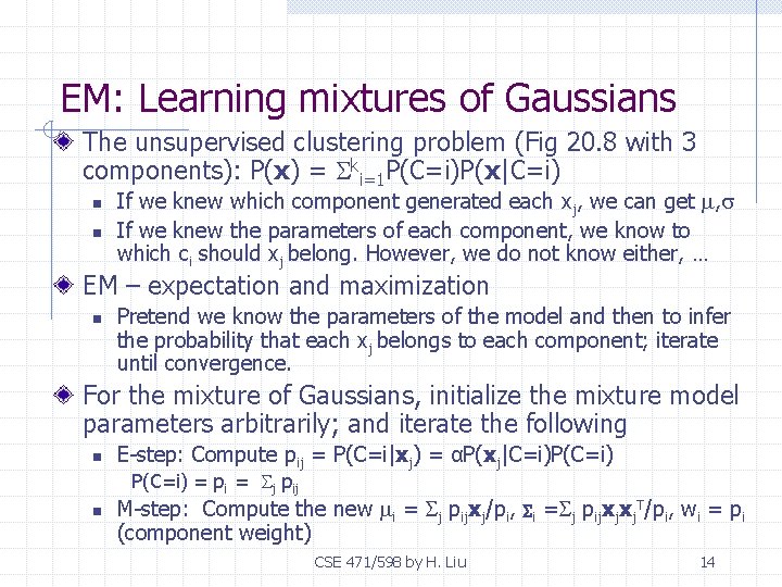
EM: Learning mixtures of Gaussians The unsupervised clustering problem (Fig 20. 8 with 3 components): P(x) = ki=1 P(C=i)P(x|C=i) n n If we knew which component generated each xj, we can get , If we knew the parameters of each component, we know to which ci should xj belong. However, we do not know either, … EM – expectation and maximization n Pretend we know the parameters of the model and then to infer the probability that each xj belongs to each component; iterate until convergence. For the mixture of Gaussians, initialize the mixture model parameters arbitrarily; and iterate the following n E-step: Compute pij = P(C=i|xj) = αP(xj|C=i)P(C=i) = pi = j pij n M-step: Compute the new i = j pijxj/pi, (component weight) CSE 471/598 by H. Liu i = j pijxjxj. T/pi, wi = pi 14

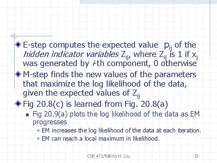
E-step computes the expected value pij of the hidden indicator variables Zij, where Zij is 1 if xj was generated by i-th component, 0 otherwise M-step finds the new values of the parameters that maximize the log likelihood of the data, given the expected values of Zij Fig 20. 8(c) is learned from Fig. 20. 8(a) n Fig 20. 9(a) plots the log likelihood of the data as EM progresses w EM increases the log likelihood of the data at each iteration. w EM can reach a local maximum in likelihood. CSE 471/598 by H. Liu 15

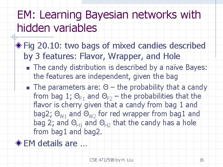
EM: Learning Bayesian networks with hidden variables Fig 20. 10: two bags of mixed candies described by 3 features: Flavor, Wrapper, and Hole n n The candy distribution is described by a naïve Bayes: the features are independent, given the bag The parameters are: Θ – the probability that a candy from bag 1; ΘF 1 and ΘF 2 – the probabilities that the flavor is cherry given that a candy from bag 1 and bag 2; ΘW 1 and ΘW 2 for red wrapper from bag 1 and bag 2; and ΘH 1 and ΘH 2 that the candy has a hole from bag 1 and bag 2. EM details are … CSE 471/598 by H. Liu 16

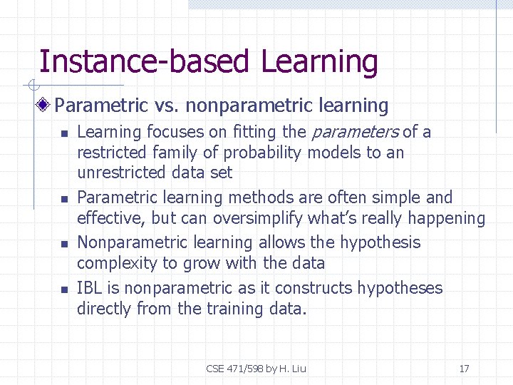
Instance-based Learning Parametric vs. nonparametric learning n n Learning focuses on fitting the parameters of a restricted family of probability models to an unrestricted data set Parametric learning methods are often simple and effective, but can oversimplify what’s really happening Nonparametric learning allows the hypothesis complexity to grow with the data IBL is nonparametric as it constructs hypotheses directly from the training data. CSE 471/598 by H. Liu 17

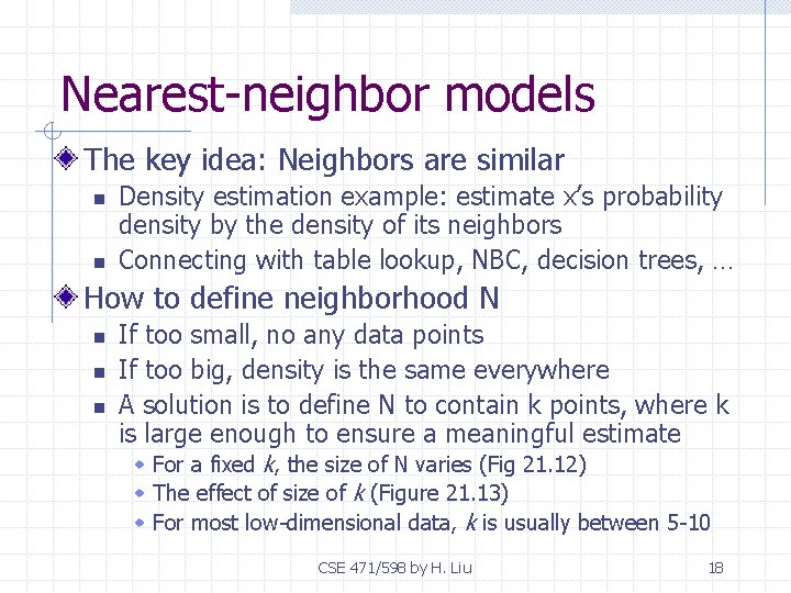
Nearest-neighbor models The key idea: Neighbors are similar n n Density estimation example: estimate x’s probability density by the density of its neighbors Connecting with table lookup, NBC, decision trees, … How to define neighborhood N n n n If too small, no any data points If too big, density is the same everywhere A solution is to define N to contain k points, where k is large enough to ensure a meaningful estimate w For a fixed k, the size of N varies (Fig 21. 12) w The effect of size of k (Figure 21. 13) w For most low-dimensional data, k is usually between 5 -10 CSE 471/598 by H. Liu 18

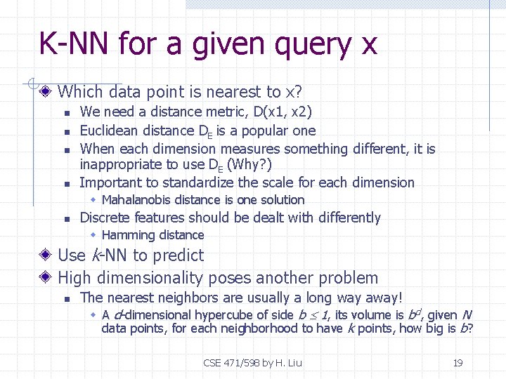
K-NN for a given query x Which data point is nearest to x? n n We need a distance metric, D(x 1, x 2) Euclidean distance DE is a popular one When each dimension measures something different, it is inappropriate to use DE (Why? ) Important to standardize the scale for each dimension w Mahalanobis distance is one solution n Discrete features should be dealt with differently w Hamming distance Use k-NN to predict High dimensionality poses another problem n The nearest neighbors are usually a long way away! w A d-dimensional hypercube of side b 1, its volume is bd, given N data points, for each neighborhood to have k points, how big is b? CSE 471/598 by H. Liu 19

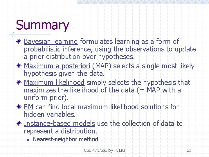
Summary Bayesian learning formulates learning as a form of probabilistic inference, using the observations to update a prior distribution over hypotheses. Maximum a posteriori (MAP) selects a single most likely hypothesis given the data. Maximum likelihood simply selects the hypothesis that maximizes the likelihood of the data (= MAP with a uniform prior). EM can find local maximum likelihood solutions for hidden variables. Instance-based models use the collection of data to represent a distribution. n Nearest-neighbor method CSE 471/598 by H. Liu 20