Statistical Learning Dong Liu Dept EEIS USTC Chapter

Statistical Learning Dong Liu Dept. EEIS, USTC

Chapter 9. Probabilistic Graphical Model 1. 2. 3. 4. 5. Generative and Bayesian Naïve Bayesian network Markov random field Belief propagation 2020/10/7 Chap 9. Probabilistic Graphical Model 2

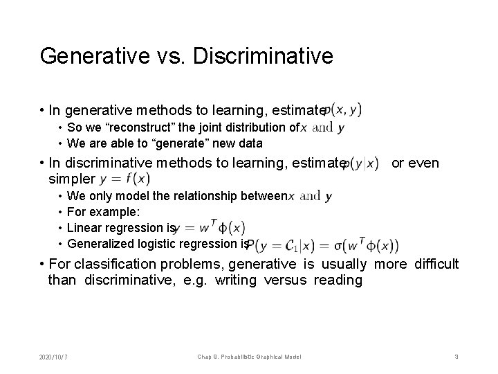
Generative vs. Discriminative • In generative methods to learning, estimate • So we “reconstruct” the joint distribution of • We are able to “generate” new data • In discriminative methods to learning, estimate simpler • • or even We only model the relationship between For example: Linear regression is Generalized logistic regression is • For classification problems, generative is usually more difficult than discriminative, e. g. writing versus reading 2020/10/7 Chap 9. Probabilistic Graphical Model 3

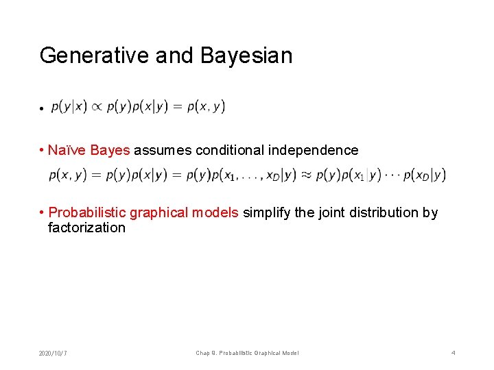
Generative and Bayesian • • Naïve Bayes assumes conditional independence • Probabilistic graphical models simplify the joint distribution by factorization 2020/10/7 Chap 9. Probabilistic Graphical Model 4

Chapter 9. Probabilistic Graphical Model 1. 2. 3. 4. 5. Generative and Bayesian Naïve Bayesian network Markov random field Belief propagation 2020/10/7 Chap 9. Probabilistic Graphical Model 5

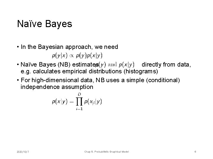
Naïve Bayes • In the Bayesian approach, we need • Naïve Bayes (NB) estimates directly from data, e. g. calculates empirical distributions (histograms) • For high-dimensional data, NB uses a simple (conditional) independence assumption 2020/10/7 Chap 9. Probabilistic Graphical Model 6

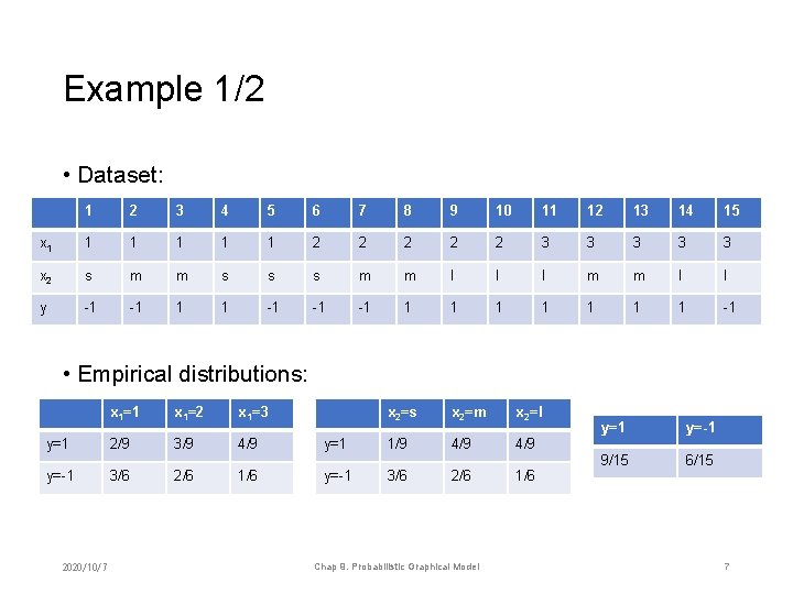
Example 1/2 • Dataset: 1 2 3 4 5 6 7 8 9 10 11 12 13 14 15 x 1 1 1 2 2 2 3 3 3 x 2 s m m s s s m m l l l m m l l y -1 -1 1 1 -1 -1 -1 1 1 1 -1 • Empirical distributions: x 1=1 x 1=2 x 1=3 y=1 2/9 3/9 4/9 y=-1 3/6 2/6 1/6 2020/10/7 x 2=s x 2=m x 2=l y=1 1/9 4/9 y=-1 3/6 2/6 1/6 Chap 9. Probabilistic Graphical Model y=1 y=-1 9/15 6/15 7

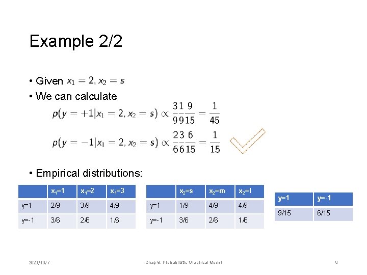
Example 2/2 • Given • We can calculate • Empirical distributions: x 1=1 x 1=2 x 1=3 y=1 2/9 3/9 4/9 y=-1 3/6 2/6 1/6 2020/10/7 x 2=s x 2=m x 2=l y=1 1/9 4/9 y=-1 3/6 2/6 1/6 Chap 9. Probabilistic Graphical Model y=1 y=-1 9/15 6/15 8

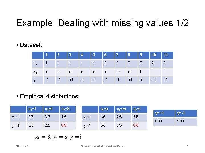
Example: Dealing with missing values 1/2 • Dataset: 1 2 3 4 5 6 7 8 9 10 11 x 1 1 1 2 2 2 3 x 2 s m m s s s m m l l l y -1 -1 +1 +1 -1 -1 -1 +1 +1 • Empirical distributions: x 1=1 x 1=2 x 1=3 y=+1 2/6 3/6 1/6 y=-1 3/5 2/5 0/5 2020/10/7 x 2=s x 2=m x 2=l y=+1 1/6 2/6 3/6 y=-1 3/5 2/5 0/5 Chap 9. Probabilistic Graphical Model y=+1 y=-1 6/11 5/11 9

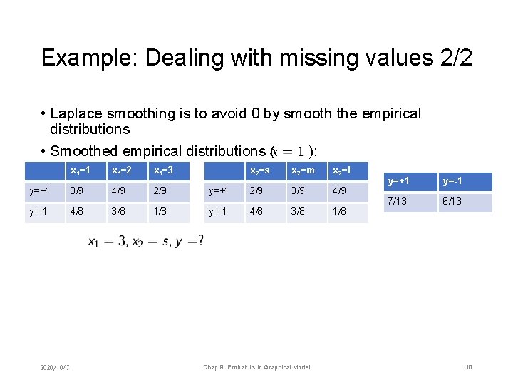
Example: Dealing with missing values 2/2 • Laplace smoothing is to avoid 0 by smooth the empirical distributions • Smoothed empirical distributions ( ): x 1=1 x 1=2 x 1=3 y=+1 3/9 4/9 2/9 y=-1 4/8 3/8 1/8 2020/10/7 x 2=s x 2=m x 2=l y=+1 2/9 3/9 4/9 y=-1 4/8 3/8 1/8 Chap 9. Probabilistic Graphical Model y=+1 y=-1 7/13 6/13 10

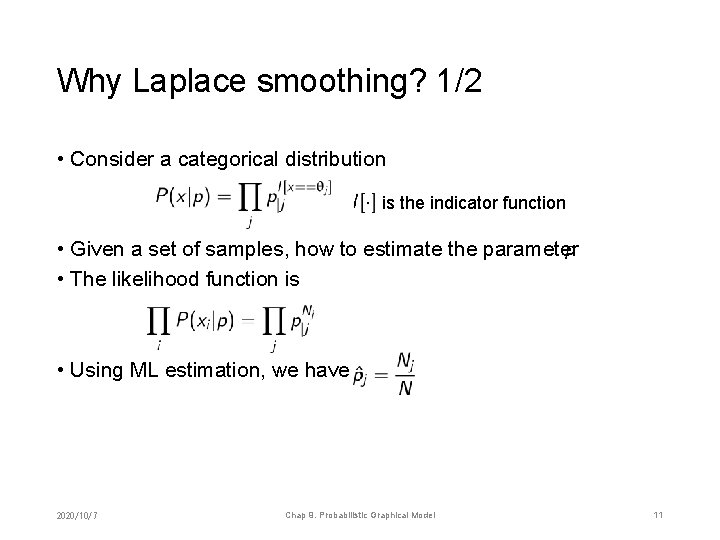
Why Laplace smoothing? 1/2 • Consider a categorical distribution is the indicator function • Given a set of samples, how to estimate the parameter • The likelihood function is • Using ML estimation, we have 2020/10/7 Chap 9. Probabilistic Graphical Model 11

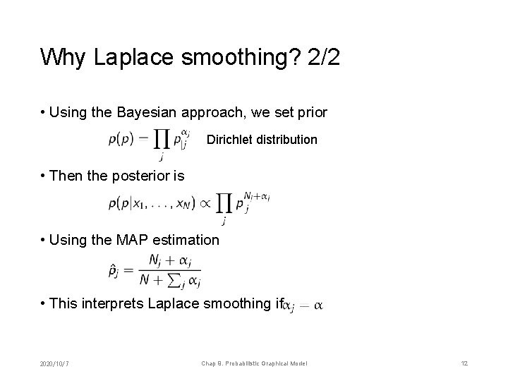
Why Laplace smoothing? 2/2 • Using the Bayesian approach, we set prior Dirichlet distribution • Then the posterior is • Using the MAP estimation • This interprets Laplace smoothing if 2020/10/7 Chap 9. Probabilistic Graphical Model 12

Notes • Naïve Bayes is especially suitable for discrete variables, so it is more used for classification 2020/10/7 Chap 9. Probabilistic Graphical Model 13

Chapter 9. Probabilistic Graphical Model 1. 2. 3. 4. 5. Generative and Bayesian Naïve Bayesian network Markov random field Belief propagation 2020/10/7 Chap 9. Probabilistic Graphical Model 14

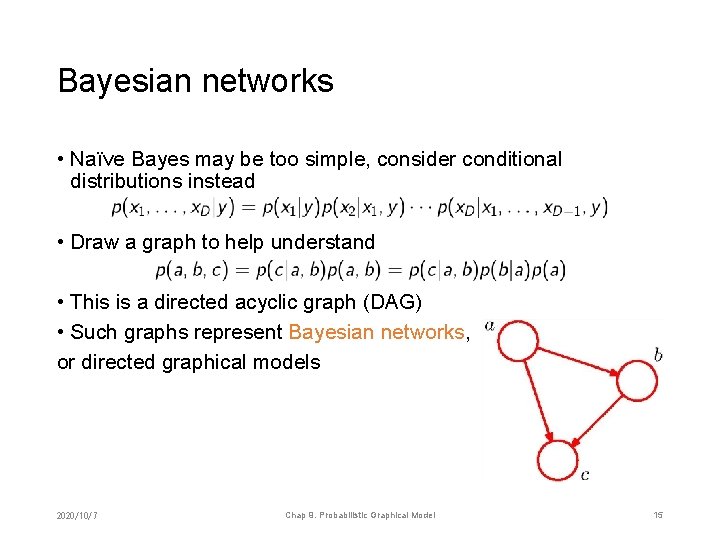
Bayesian networks • Naïve Bayes may be too simple, consider conditional distributions instead • Draw a graph to help understand • This is a directed acyclic graph (DAG) • Such graphs represent Bayesian networks, or directed graphical models 2020/10/7 Chap 9. Probabilistic Graphical Model 15

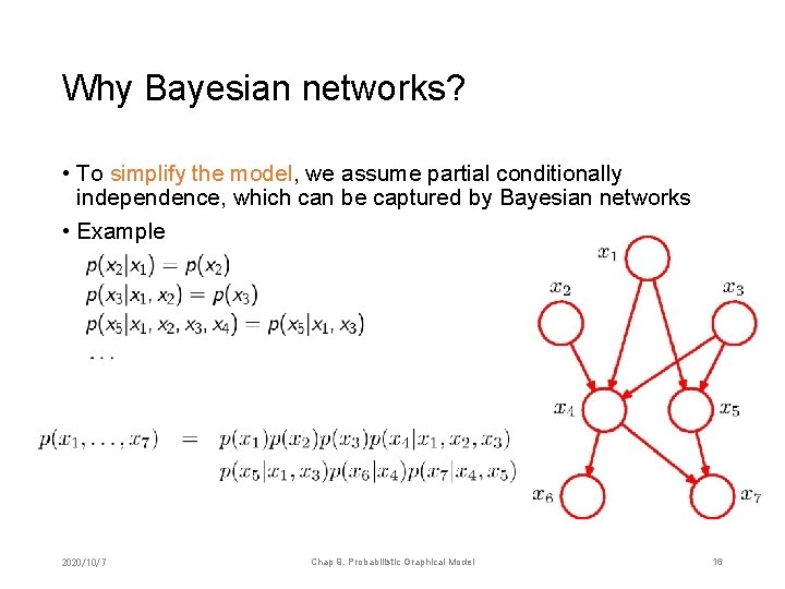
Why Bayesian networks? • To simplify the model, we assume partial conditionally independence, which can be captured by Bayesian networks • Example 2020/10/7 Chap 9. Probabilistic Graphical Model 16

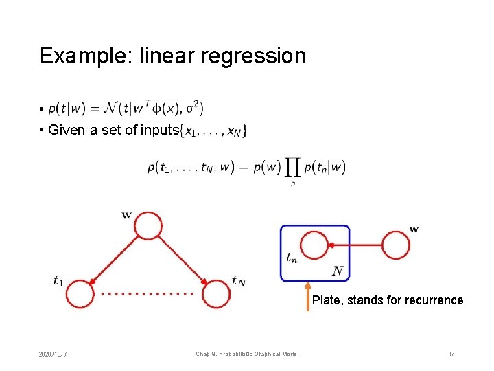
Example: linear regression • • Given a set of inputs Plate, stands for recurrence 2020/10/7 Chap 9. Probabilistic Graphical Model 17

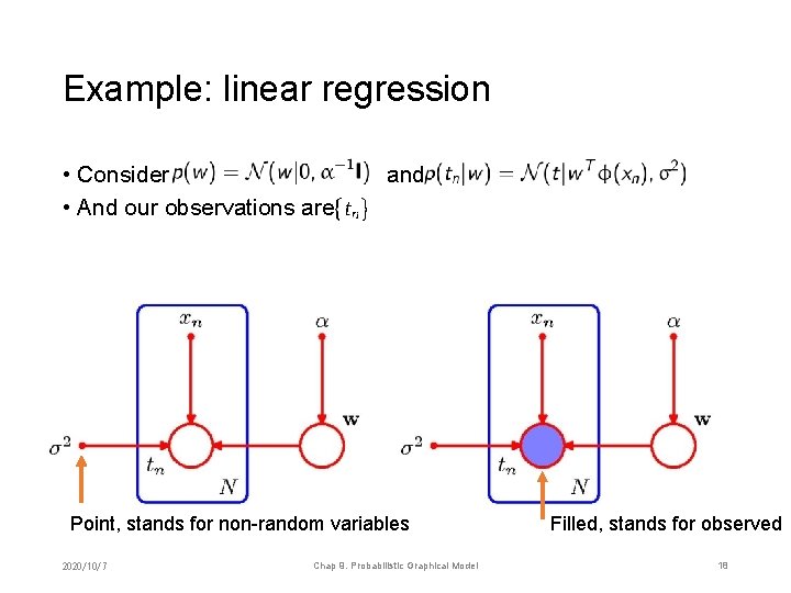
Example: linear regression • Consider • And our observations are and Point, stands for non-random variables 2020/10/7 Chap 9. Probabilistic Graphical Model Filled, stands for observed 18

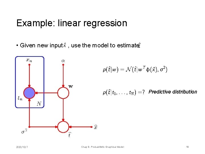
Example: linear regression • Given new input , use the model to estimate Predictive distribution 2020/10/7 Chap 9. Probabilistic Graphical Model 19

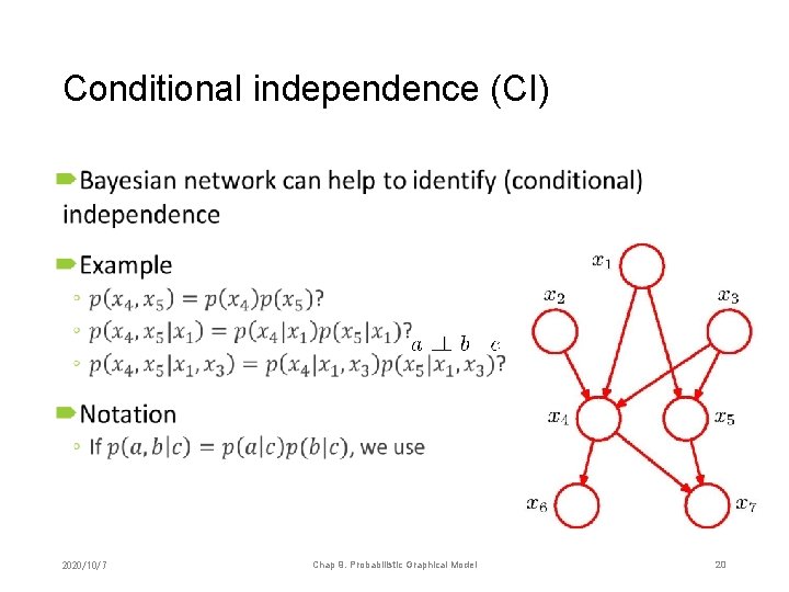
Conditional independence (CI) • 2020/10/7 Chap 9. Probabilistic Graphical Model 20

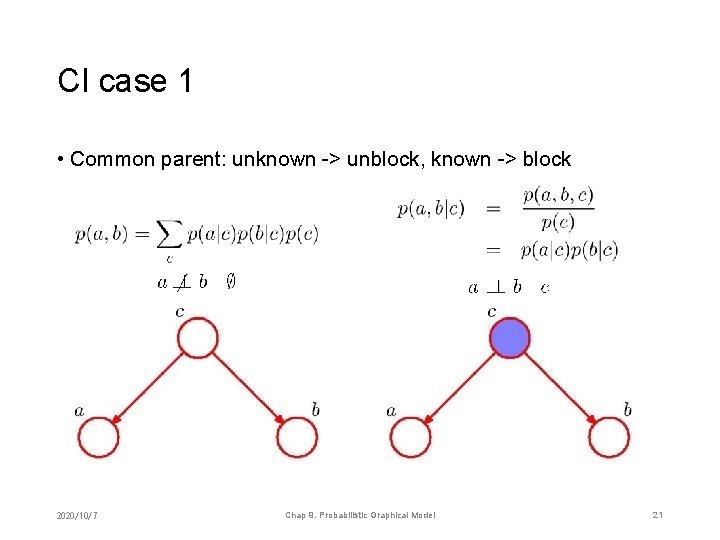
CI case 1 • Common parent: unknown -> unblock, known -> block 2020/10/7 Chap 9. Probabilistic Graphical Model 21

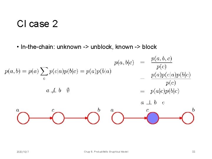
CI case 2 • In-the-chain: unknown -> unblock, known -> block 2020/10/7 Chap 9. Probabilistic Graphical Model 22

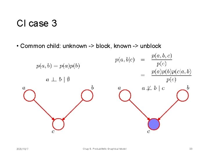
CI case 3 • Common child: unknown -> block, known -> unblock 2020/10/7 Chap 9. Probabilistic Graphical Model 23

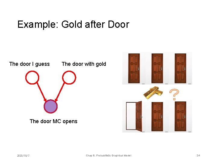
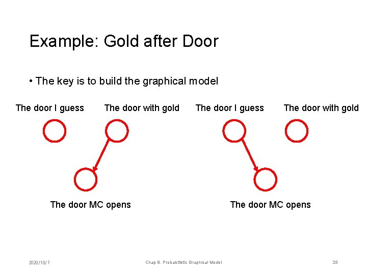
Example: Gold after Door The door I guess The door with gold ？ The door MC opens 2020/10/7 Chap 9. Probabilistic Graphical Model 24

Example: Gold after Door • The key is to build the graphical model The door I guess The door with gold The door I guess The door MC opens 2020/10/7 The door with gold The door MC opens Chap 9. Probabilistic Graphical Model 25

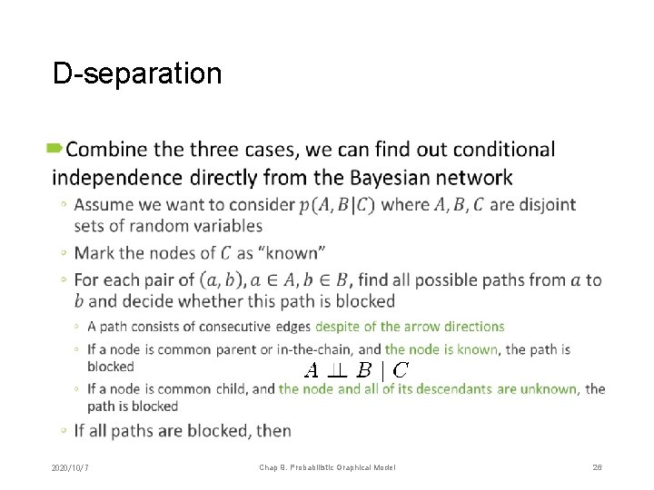
D-separation • 2020/10/7 Chap 9. Probabilistic Graphical Model 26

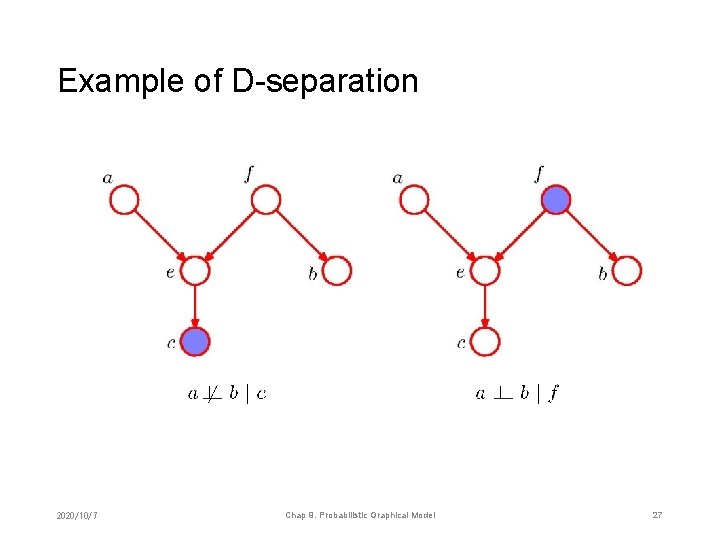
Example of D-separation 2020/10/7 Chap 9. Probabilistic Graphical Model 27

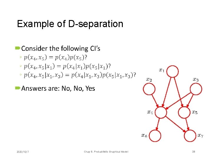
Example of D-separation • 2020/10/7 Chap 9. Probabilistic Graphical Model 28

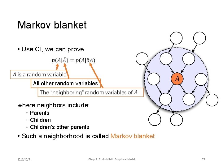
Markov blanket • Use CI, we can prove All other random variables where neighbors include: • Parents • Children’s other parents • Such a neighborhood is called Markov blanket 2020/10/7 Chap 9. Probabilistic Graphical Model 29

Chapter 9. Probabilistic Graphical Model 1. 2. 3. 4. 5. Generative and Bayesian Naïve Bayesian network Markov random field Belief propagation 2020/10/7 Chap 9. Probabilistic Graphical Model 30

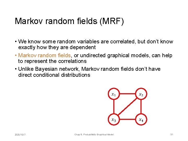
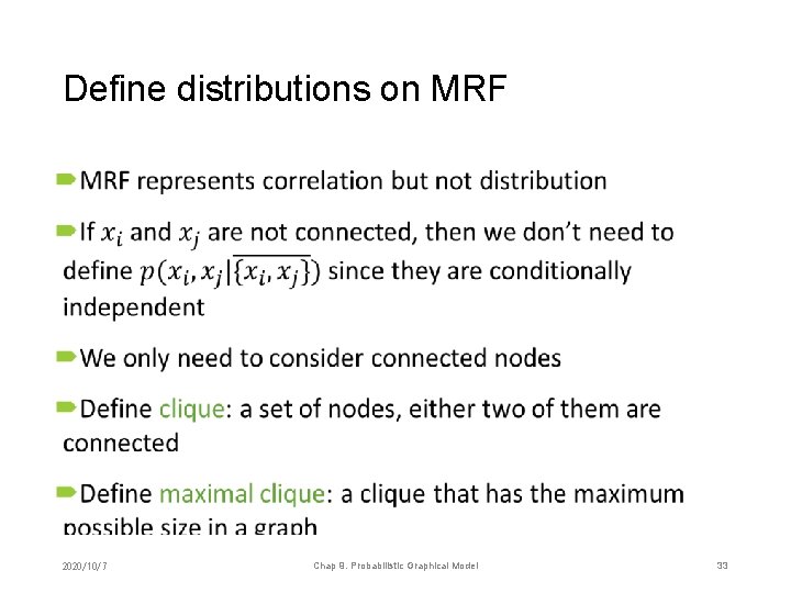
Markov random fields (MRF) • We know some random variables are correlated, but don’t know exactly how they are dependent • Markov random fields, or undirected graphical models, can help to represent the correlations • Unlike Bayesian network, Markov random fields don’t have direct conditional distributions 2020/10/7 Chap 9. Probabilistic Graphical Model 31

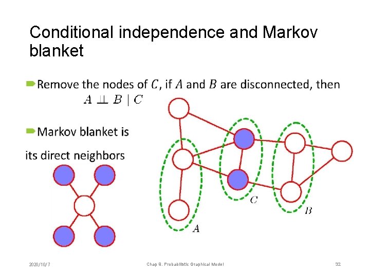
Conditional independence and Markov blanket • 2020/10/7 Chap 9. Probabilistic Graphical Model 32

Define distributions on MRF • 2020/10/7 Chap 9. Probabilistic Graphical Model 33

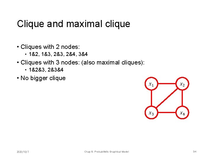
Clique and maximal clique • Cliques with 2 nodes: • 1&2, 1&3, 2&4, 3&4 • Cliques with 3 nodes: (also maximal cliques): • 1&2&3, 2&3&4 • No bigger clique 2020/10/7 Chap 9. Probabilistic Graphical Model 34

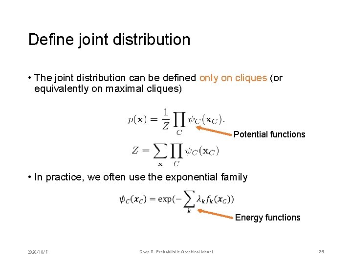
Define joint distribution • The joint distribution can be defined only on cliques (or equivalently on maximal cliques) Potential functions • In practice, we often use the exponential family Energy functions 2020/10/7 Chap 9. Probabilistic Graphical Model 35

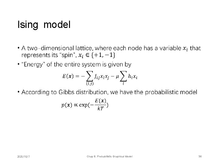
Ising model • 2020/10/7 Chap 9. Probabilistic Graphical Model 36

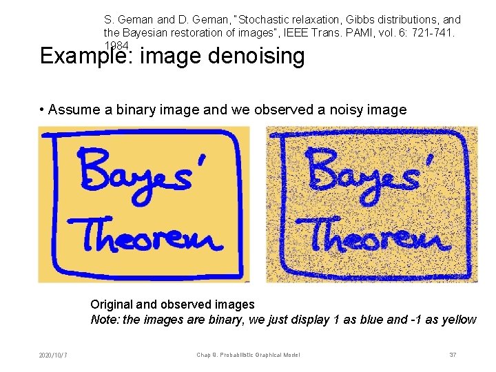
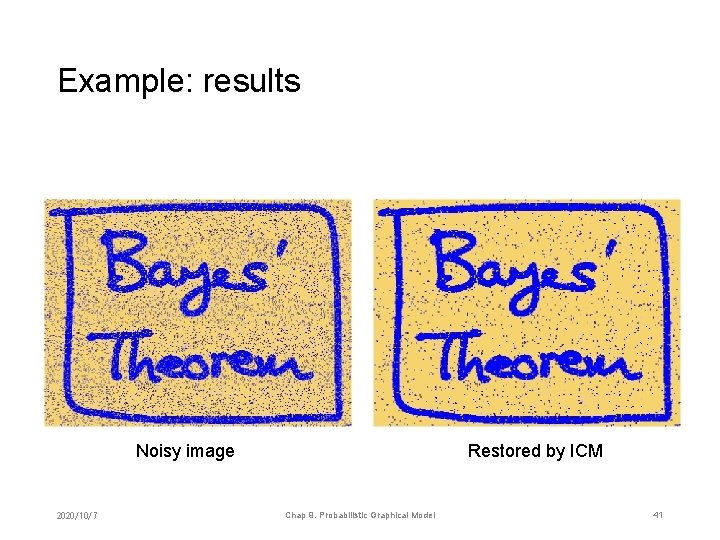
S. Geman and D. Geman, “Stochastic relaxation, Gibbs distributions, and the Bayesian restoration of images”, IEEE Trans. PAMI, vol. 6: 721 -741. 1984 Example: image denoising • Assume a binary image and we observed a noisy image Original and observed images Note: the images are binary, we just display 1 as blue and -1 as yellow 2020/10/7 Chap 9. Probabilistic Graphical Model 37

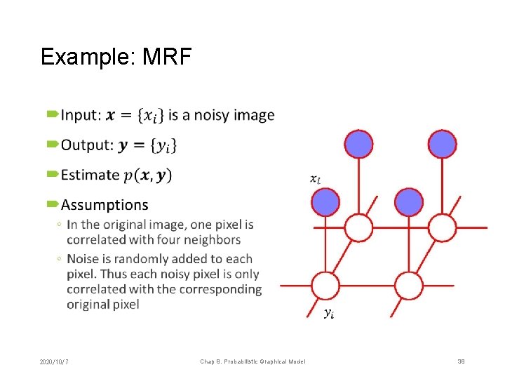
Example: MRF • 2020/10/7 Chap 9. Probabilistic Graphical Model 38

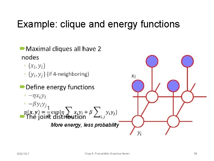
Example: clique and energy functions • More energy, less probability 2020/10/7 Chap 9. Probabilistic Graphical Model 39

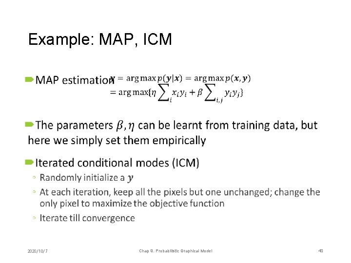
Example: MAP, ICM • 2020/10/7 Chap 9. Probabilistic Graphical Model 40

Example: results Noisy image 2020/10/7 Restored by ICM Chap 9. Probabilistic Graphical Model 41

BN vs. MRF Bayesian networks Markov Random Fields • Directed graphical models • Modeling conditional probabilities • CI: D-separation • Markov blanket: parents, children’s other parents • Undirected graphical models • Modeling correlations, need to define probability functions • CI: simple connection • Markov blanket: directly connected nodes 2020/10/7 Chap 9. Probabilistic Graphical Model 42

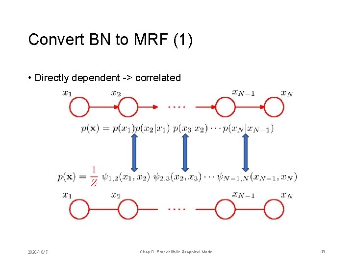
Convert BN to MRF (1) • Directly dependent -> correlated 2020/10/7 Chap 9. Probabilistic Graphical Model 43

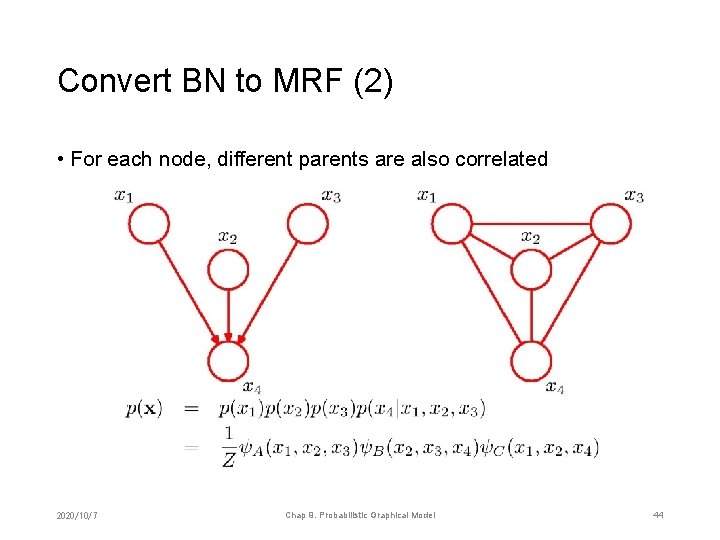
Convert BN to MRF (2) • For each node, different parents are also correlated 2020/10/7 Chap 9. Probabilistic Graphical Model 44

Convert BN to MRF - Moralization • After conversion, the Markov blanket of each node keeps unchanged; this conversion is known as moralization 2020/10/7 Chap 9. Probabilistic Graphical Model 45

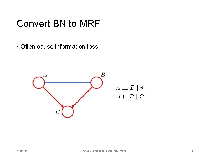
Convert BN to MRF • Often cause information loss 2020/10/7 Chap 9. Probabilistic Graphical Model 46

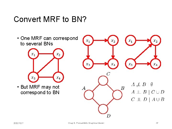
Convert MRF to BN? • One MRF can correspond to several BNs • But MRF may not correspond to BN 2020/10/7 Chap 9. Probabilistic Graphical Model 47

Chapter 9. Probabilistic Graphical Model 1. 2. 3. 4. 5. Generative and Bayesian Naïve Bayesian network Markov random field Belief propagation 2020/10/7 Chap 9. Probabilistic Graphical Model 48

Inference in graphical models • Inference of unobserved variables • Given a set of observed variables, graphical models can help to infer the posterior distributions of target variables • Need integral to eliminate “neither observed nor target” variables • Inference of conditional distributions • Inference of graph structure 2020/10/7 Chap 9. Probabilistic Graphical Model 49

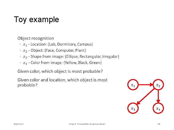
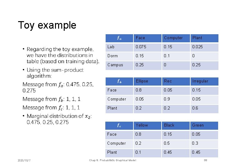
Toy example • 2020/10/7 Chap 9. Probabilistic Graphical Model 50

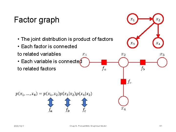
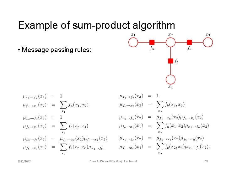
Factor graph • The joint distribution is product of factors • Each factor is connected to related variables • Each variable is connected to related factors 2020/10/7 Chap 9. Probabilistic Graphical Model 51

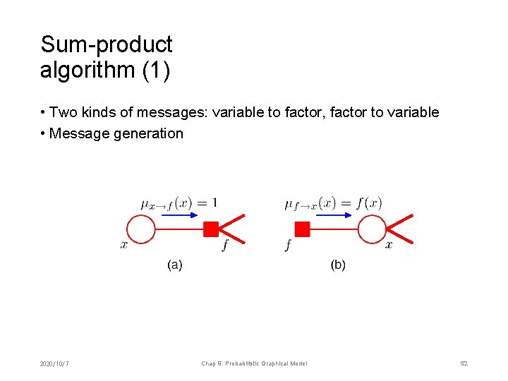
Sum-product algorithm (1) • Two kinds of messages: variable to factor, factor to variable • Message generation 2020/10/7 Chap 9. Probabilistic Graphical Model 52

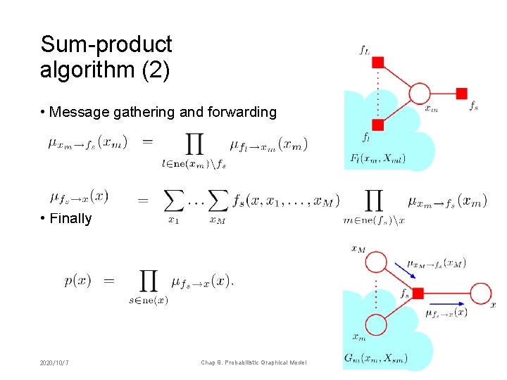
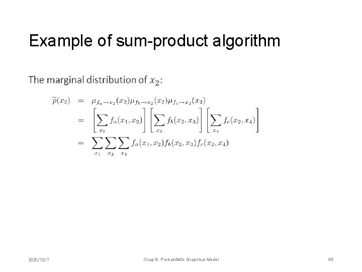
Sum-product algorithm (2) • Message gathering and forwarding • Finally 2020/10/7 Chap 9. Probabilistic Graphical Model 53

Example of sum-product algorithm • Message passing rules: 2020/10/7 Chap 9. Probabilistic Graphical Model 54

Example of sum-product algorithm • 2020/10/7 Chap 9. Probabilistic Graphical Model 55

Toy example • 2020/10/7 Face Computer Plant Lab 0. 075 0. 15 0. 025 Dorm 0. 15 0. 1 0 Campus 0. 25 0 0. 25 Ellipse Rec Irregular Face 0. 8 0. 05 0. 15 Computer 0. 05 0. 9 0. 05 Plant 0. 2 0. 6 Yellow Black Green Face 0. 8 0. 15 0. 05 Computer 0. 2 0. 5 0. 3 Plant 0. 1 0. 45 Chap 9. Probabilistic Graphical Model 56

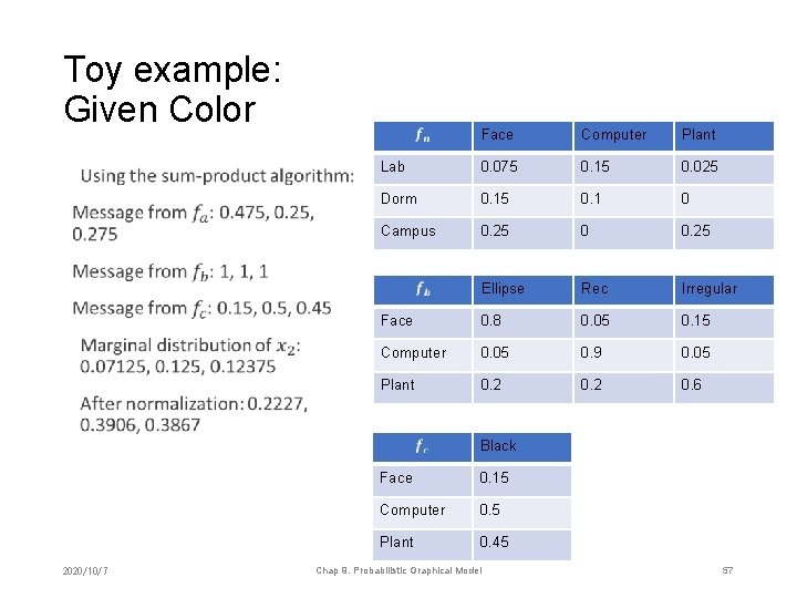
Toy example: Given Color • Face Computer Plant Lab 0. 075 0. 15 0. 025 Dorm 0. 15 0. 1 0 Campus 0. 25 0 0. 25 Ellipse Rec Irregular Face 0. 8 0. 05 0. 15 Computer 0. 05 0. 9 0. 05 Plant 0. 2 0. 6 Black 2020/10/7 Face 0. 15 Computer 0. 5 Plant 0. 45 Chap 9. Probabilistic Graphical Model 57

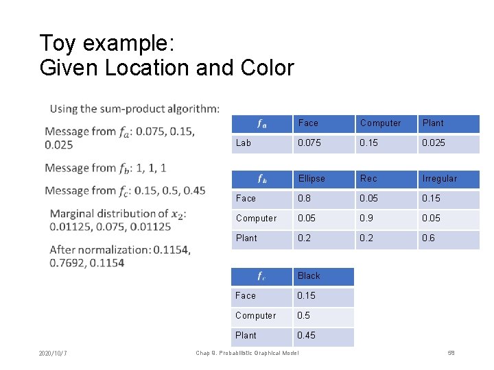
Toy example: Given Location and Color • Face Computer Plant 0. 075 0. 15 0. 025 Ellipse Rec Irregular Face 0. 8 0. 05 0. 15 Computer 0. 05 0. 9 0. 05 Plant 0. 2 0. 6 Lab Black 2020/10/7 Face 0. 15 Computer 0. 5 Plant 0. 45 Chap 9. Probabilistic Graphical Model 58

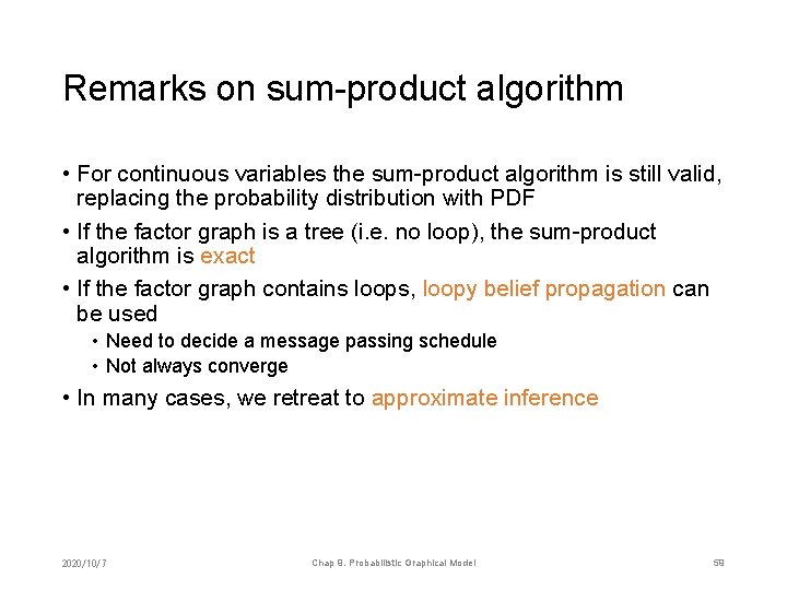
Remarks on sum-product algorithm • For continuous variables the sum-product algorithm is still valid, replacing the probability distribution with PDF • If the factor graph is a tree (i. e. no loop), the sum-product algorithm is exact • If the factor graph contains loops, loopy belief propagation can be used • Need to decide a message passing schedule • Not always converge • In many cases, we retreat to approximate inference 2020/10/7 Chap 9. Probabilistic Graphical Model 59

Chapter summary Dictionary Toolbox • Bayesian network • Factor graph • Graphical model • Markov blanket • Markov random field (MRF) • Belief propagation, aka sumproduct algorithm, aka message passing, loopy ~ • D-separation • Iterative conditional modes (ICM) • Laplace smoothing • Moralization • Naïve Bayes 2020/10/7 Chap 5. Non-Parametric Supervised Learning 60

Home exercises 2020/10/7 Chap 1. Linear Regression 61