Statistical Inference Making decisions regarding the population base

Statistical Inference Making decisions regarding the population base on a sample

Decision Types • Estimation – Deciding on the value of an unknown parameter • Hypothesis Testing – Deciding a statement regarding an unknown parameter is true of false • All decisions will be based on the values of statistics

Estimation • Definitions – An estimator of an unknown parameter is a sample statistic used for this purpose – An estimate is the value of the estimator after the data is collected • The performance of an estimator is assessed by determining its sampling distribution and measuring its closeness to the parameter being estimated

Examples of Estimators

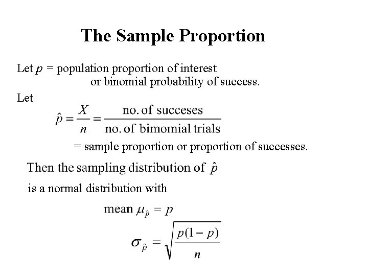
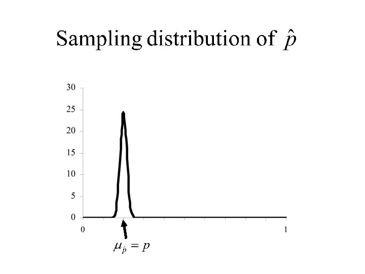
The Sample Proportion Let p = population proportion of interest or binomial probability of success. Let = sample proportion or proportion of successes. is a normal distribution with

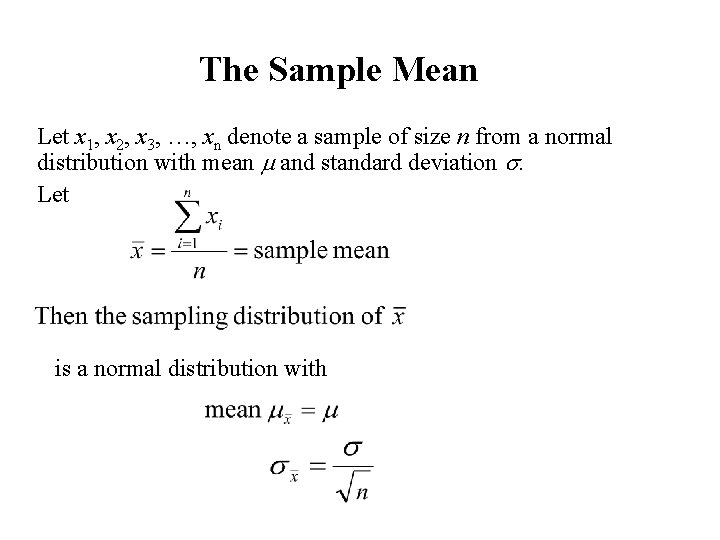
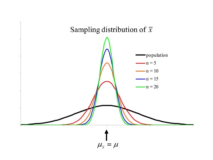
The Sample Mean Let x 1, x 2, x 3, …, xn denote a sample of size n from a normal distribution with mean m and standard deviation s. Let is a normal distribution with

Confidence Intervals

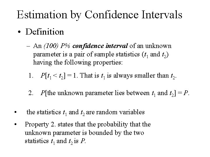
Estimation by Confidence Intervals • Definition – An (100) P% confidence interval of an unknown parameter is a pair of sample statistics (t 1 and t 2) having the following properties: 1. P[t 1 < t 2] = 1. That is t 1 is always smaller than t 2. 2. P[the unknown parameter lies between t 1 and t 2] = P. • the statistics t 1 and t 2 are random variables • Property 2. states that the probability that the unknown parameter is bounded by the two statistics t 1 and t 2 is P.

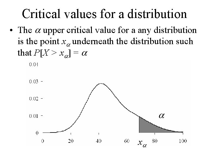
Critical values for a distribution • The a upper critical value for a any distribution is the point xa underneath the distribution such that P[X > xa] = a a xa

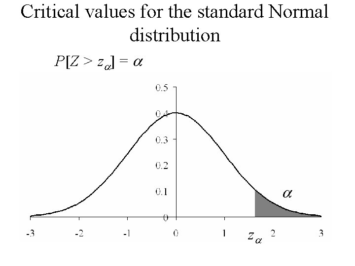
Critical values for the standard Normal distribution P[Z > za] = a a za

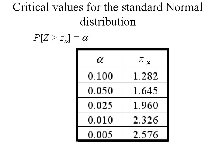
Critical values for the standard Normal distribution P[Z > za] = a

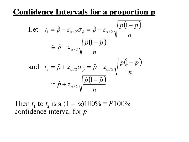
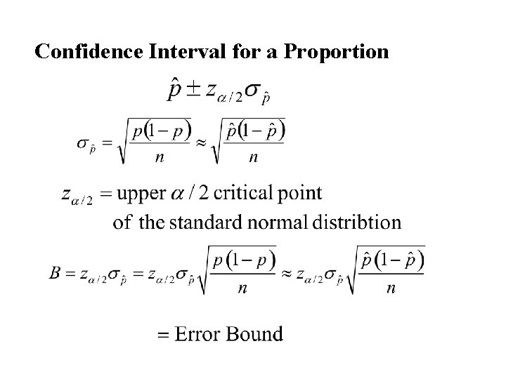
Confidence Intervals for a proportion p Let and Then t 1 to t 2 is a (1 – a)100% = P 100% confidence interval for p

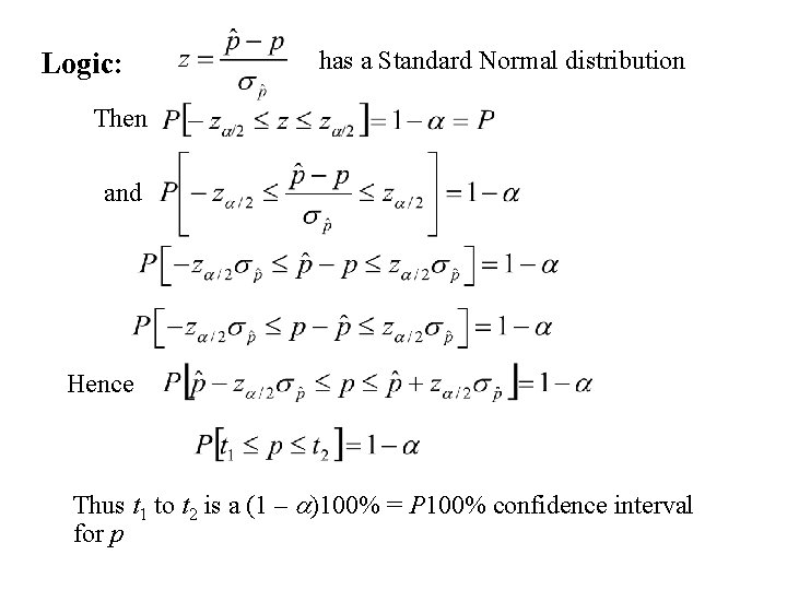
Logic: has a Standard Normal distribution Then and Hence Thus t 1 to t 2 is a (1 – a)100% = P 100% confidence interval for p

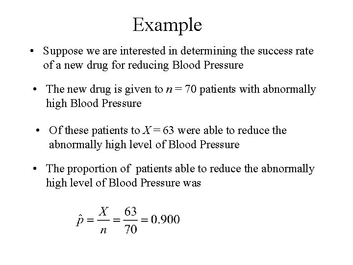
Example • Suppose we are interested in determining the success rate of a new drug for reducing Blood Pressure • The new drug is given to n = 70 patients with abnormally high Blood Pressure • Of these patients to X = 63 were able to reduce the abnormally high level of Blood Pressure • The proportion of patients able to reduce the abnormally high level of Blood Pressure was

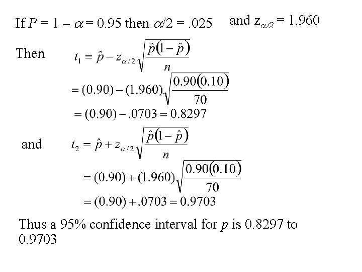
If P = 1 – a = 0. 95 then a/2 =. 025 and za/2 = 1. 960 Then and Thus a 95% confidence interval for p is 0. 8297 to 0. 9703

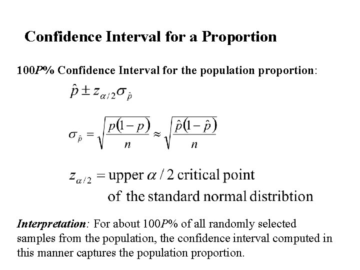
Confidence Interval for a Proportion 100 P% Confidence Interval for the population proportion: Interpretation: For about 100 P% of all randomly selected samples from the population, the confidence interval computed in this manner captures the population proportion.

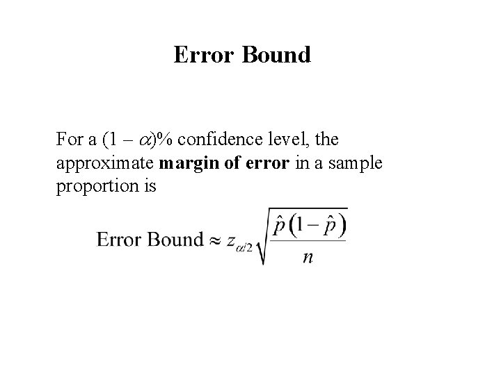
Error Bound For a (1 – a)% confidence level, the approximate margin of error in a sample proportion is

Factors that Determine the Error Bound 1. The sample size, n. When sample size increases, margin of error decreases. 2. The sample proportion, . If the proportion is close to either 1 or 0 most individuals have the same trait or opinion, so there is little natural variability and the margin of error is smaller than if the proportion is near 0. 5. 3. The “multiplier” za/2. Connected to the “(1 – a)%” level of confindence of the Error Bound. The value of za/2 for a 95% level of confidence is 1. 96 This value is changed to change the level of confidence.

Determination of Sample Size In almost all research situations the researcher is interested in the question: How large should the sample be?

Answer: Depends on: • How accurate you want the answer. Accuracy is specified by: • Specifying the magnitude of the error bound • Level of confidence

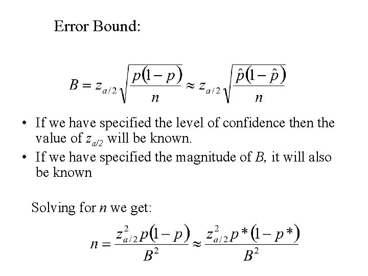
Error Bound: • If we have specified the level of confidence then the value of za/2 will be known. • If we have specified the magnitude of B, it will also be known Solving for n we get:

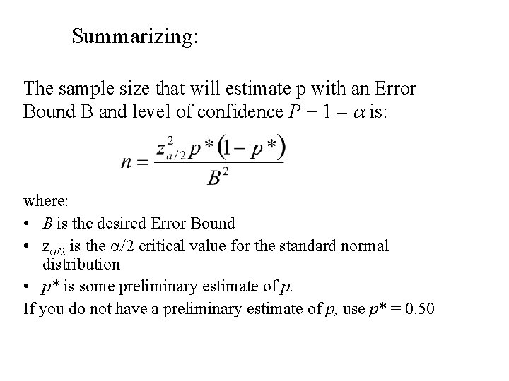
Summarizing: The sample size that will estimate p with an Error Bound B and level of confidence P = 1 – a is: where: • B is the desired Error Bound • za/2 is the a/2 critical value for the standard normal distribution • p* is some preliminary estimate of p. If you do not have a preliminary estimate of p, use p* = 0. 50

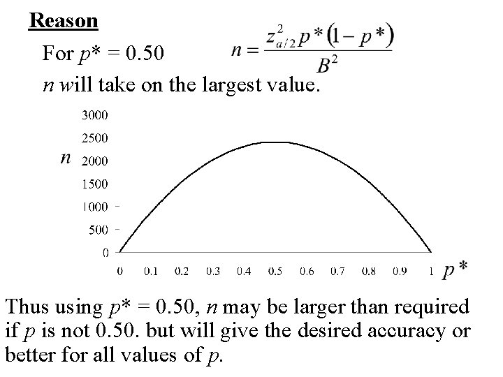
Reason For p* = 0. 50 n will take on the largest value. Thus using p* = 0. 50, n may be larger than required if p is not 0. 50. but will give the desired accuracy or better for all values of p.

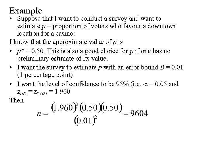
Example • Suppose that I want to conduct a survey and want to estimate p = proportion of voters who favour a downtown location for a casino: I know that the approximate value of p is • p* = 0. 50. This is also a good choice for p if one has no preliminary estimate of its value. • I want the survey to estimate p with an error bound B = 0. 01 (1 percentage point) • I want the level of confidence to be 95% (i. e. a = 0. 05 and za/2 = z 0. 025 = 1. 960 Then

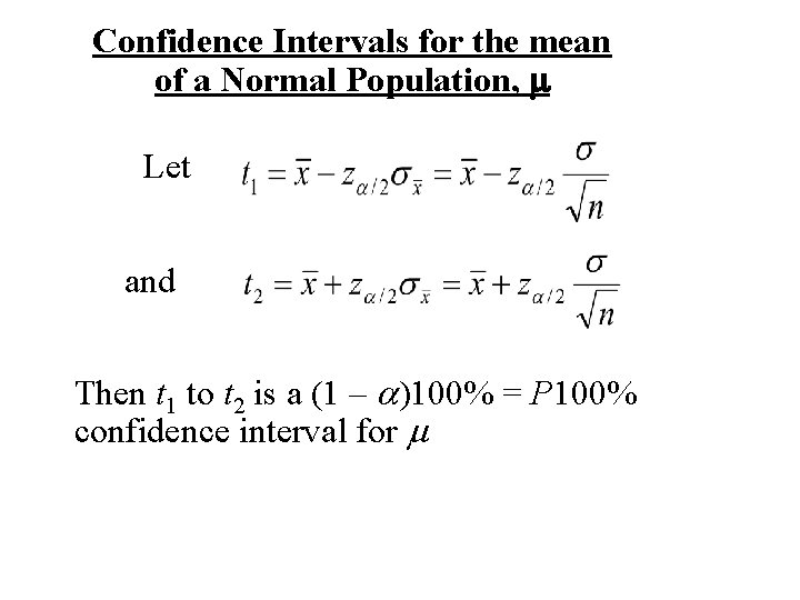
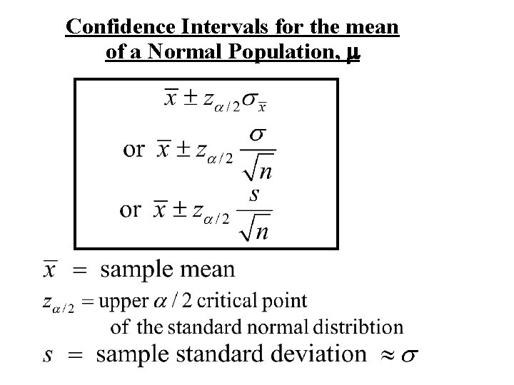
Confidence Intervals for the mean of a Normal Population, m Let and Then t 1 to t 2 is a (1 – a)100% = P 100% confidence interval for m

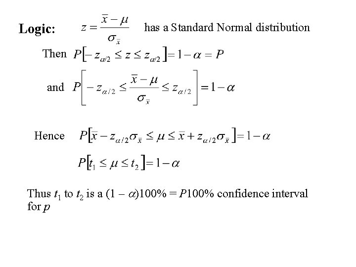
Logic: has a Standard Normal distribution Then and Hence Thus t 1 to t 2 is a (1 – a)100% = P 100% confidence interval for p

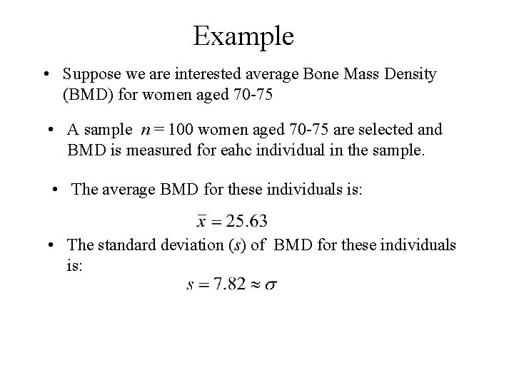
Example • Suppose we are interested average Bone Mass Density (BMD) for women aged 70 -75 • A sample n = 100 women aged 70 -75 are selected and BMD is measured for eahc individual in the sample. • The average BMD for these individuals is: • The standard deviation (s) of BMD for these individuals is:

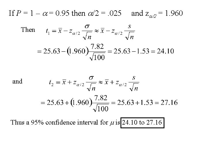
If P = 1 – a = 0. 95 then a/2 =. 025 and za/2 = 1. 960 Then and Thus a 95% confidence interval for m is 24. 10 to 27. 16

Determination of Sample Size Again a question to be asked: How large should the sample be?

Answer: Depends on: • How accurate you want the answer. Accuracy is specified by: • Specifying the magnitude of the error bound • Level of confidence

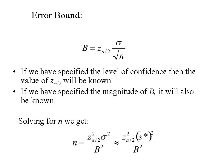
Error Bound: • If we have specified the level of confidence then the value of za/2 will be known. • If we have specified the magnitude of B, it will also be known Solving for n we get:

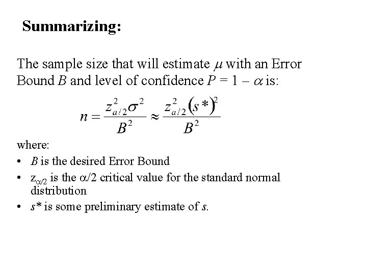
Summarizing: The sample size that will estimate m with an Error Bound B and level of confidence P = 1 – a is: where: • B is the desired Error Bound • za/2 is the a/2 critical value for the standard normal distribution • s* is some preliminary estimate of s.

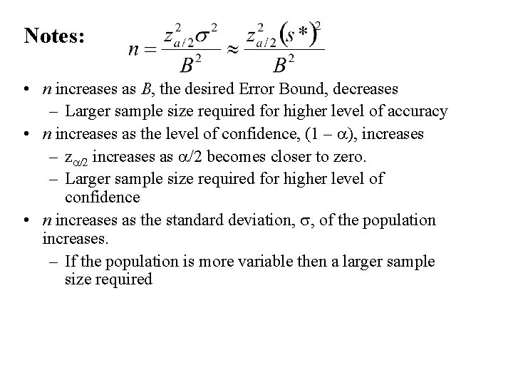
Notes: • n increases as B, the desired Error Bound, decreases – Larger sample size required for higher level of accuracy • n increases as the level of confidence, (1 – a), increases – za/2 increases as a/2 becomes closer to zero. – Larger sample size required for higher level of confidence • n increases as the standard deviation, s, of the population increases. – If the population is more variable then a larger sample size required

Summary: The sample size n depends on: • Desired level of accuracy • Desired level of confidence • Variability of the population

Example • Suppose that one is interested in estimating the average number of grams of fat (m) in one kilogram of lean beef hamburger : This will be estimated by: • randomly selecting one kilogram samples, then • Measuring the fat content for each sample. • Preliminary estimates of m and s indicate: – that m and s are approximately 220 and 40 respectively. • I want the study to estimate m with an error bound 5 and • a level of confidence to be 95% (i. e. a = 0. 05 and za/2 = z 0. 025 = 1. 960)

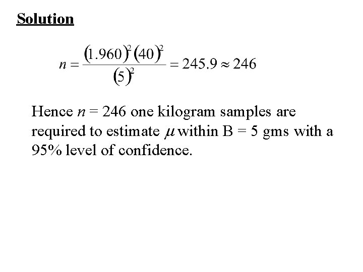
Solution Hence n = 246 one kilogram samples are required to estimate m within B = 5 gms with a 95% level of confidence.

Confidence Intervals

Confidence Interval for a Proportion

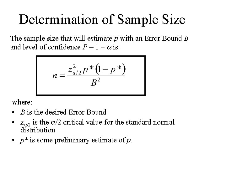
Determination of Sample Size The sample size that will estimate p with an Error Bound B and level of confidence P = 1 – a is: where: • B is the desired Error Bound • za/2 is the a/2 critical value for the standard normal distribution • p* is some preliminary estimate of p.

Confidence Intervals for the mean of a Normal Population, m

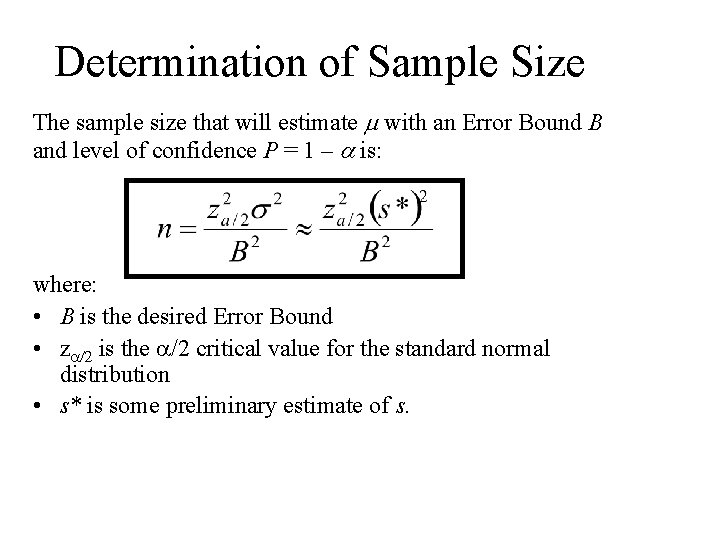
Determination of Sample Size The sample size that will estimate m with an Error Bound B and level of confidence P = 1 – a is: where: • B is the desired Error Bound • za/2 is the a/2 critical value for the standard normal distribution • s* is some preliminary estimate of s.

Hypothesis Testing An important area of statistical inference

Definition Hypothesis (H) – Statement about the parameters of the population • In hypothesis testing there are two hypotheses of interest. – The null hypothesis (H 0) – The alternative hypothesis (HA)

Either – null hypothesis (H 0) is true or – the alternative hypothesis (HA) is true. But not both We say that are mutually exclusive and exhaustive.

One has to make a decision – to either to accept null hypothesis (equivalent to rejecting HA) or – to reject null hypothesis (equivalent to accepting HA)

There are two possible errors that can be made. 1. Rejecting the null hypothesis when it is true. (type I error) 2. accepting the null hypothesis when it is false (type II error)

An analogy – a jury trial The two possible decisions are – Declare the accused innocent. – Declare the accused guilty.

The null hypothesis (H 0) – the accused is innocent The alternative hypothesis (HA) – the accused is guilty

The two possible errors that can be made: – Declaring an innocent person guilty. (type I error) – Declaring a guilty person innocent. (type II error) Note: in this case one type of error may be considered more serious

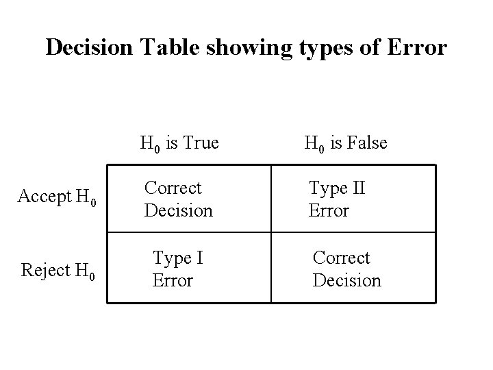
Decision Table showing types of Error H 0 is True H 0 is False Accept H 0 Correct Decision Type II Error Reject H 0 Type I Error Correct Decision

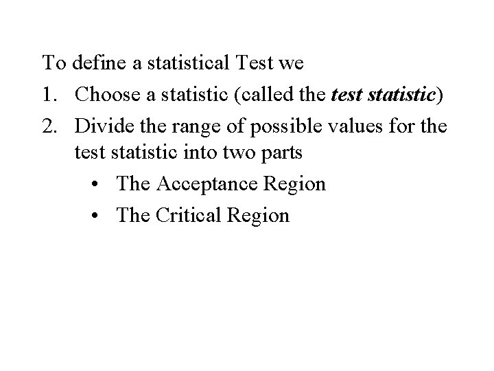
To define a statistical Test we 1. Choose a statistic (called the test statistic) 2. Divide the range of possible values for the test statistic into two parts • The Acceptance Region • The Critical Region

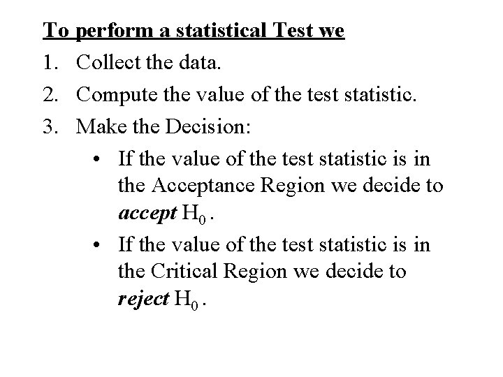
To perform a statistical Test we 1. Collect the data. 2. Compute the value of the test statistic. 3. Make the Decision: • If the value of the test statistic is in the Acceptance Region we decide to accept H 0. • If the value of the test statistic is in the Critical Region we decide to reject H 0.

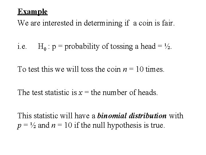
Example We are interested in determining if a coin is fair. i. e. H 0 : p = probability of tossing a head = ½. To test this we will toss the coin n = 10 times. The test statistic is x = the number of heads. This statistic will have a binomial distribution with p = ½ and n = 10 if the null hypothesis is true.

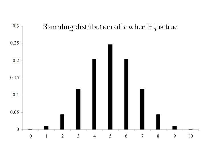
Sampling distribution of x when H 0 is true

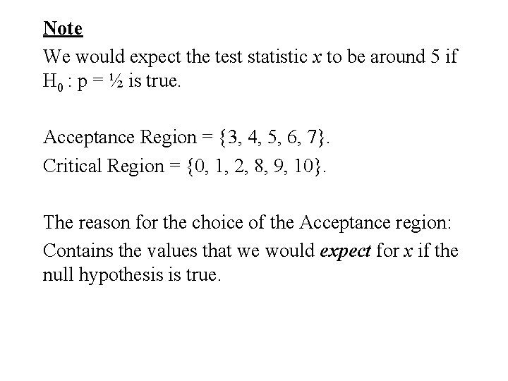
Note We would expect the test statistic x to be around 5 if H 0 : p = ½ is true. Acceptance Region = {3, 4, 5, 6, 7}. Critical Region = {0, 1, 2, 8, 9, 10}. The reason for the choice of the Acceptance region: Contains the values that we would expect for x if the null hypothesis is true.

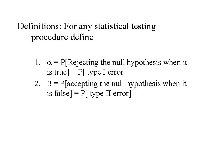
Definitions: For any statistical testing procedure define 1. a = P[Rejecting the null hypothesis when it is true] = P[ type I error] 2. b = P[accepting the null hypothesis when it is false] = P[ type II error]

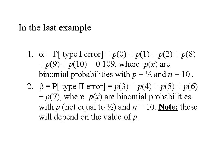
In the last example 1. a = P[ type I error] = p(0) + p(1) + p(2) + p(8) + p(9) + p(10) = 0. 109, where p(x) are binomial probabilities with p = ½ and n = 10. 2. b = P[ type II error] = p(3) + p(4) + p(5) + p(6) + p(7), where p(x) are binomial probabilities with p (not equal to ½) and n = 10. Note: these will depend on the value of p.

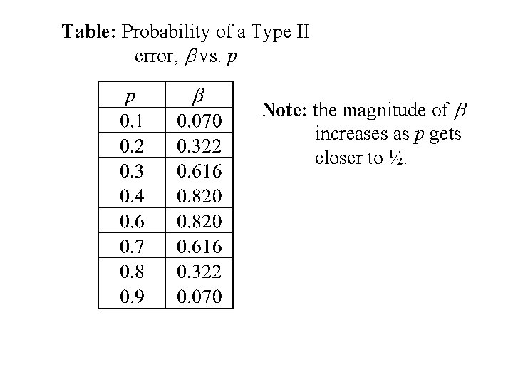
Table: Probability of a Type II error, b vs. p Note: the magnitude of b increases as p gets closer to ½.

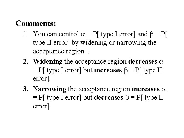
Comments: 1. You can control a = P[ type I error] and b = P[ type II error] by widening or narrowing the acceptance region. . 2. Widening the acceptance region decreases a = P[ type I error] but increases b = P[ type II error]. 3. Narrowing the acceptance region increases a = P[ type I error] but decreases b = P[ type II error].

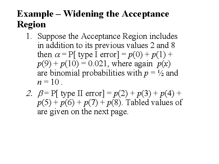
Example – Widening the Acceptance Region 1. Suppose the Acceptance Region includes in addition to its previous values 2 and 8 then a = P[ type I error] = p(0) + p(1) + p(9) + p(10) = 0. 021, where again p(x) are binomial probabilities with p = ½ and n = 10. 2. b = P[ type II error] = p(2) + p(3) + p(4) + p(5) + p(6) + p(7) + p(8). Tabled values of are given on the next page.

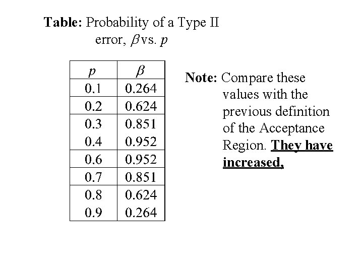
Table: Probability of a Type II error, b vs. p Note: Compare these values with the previous definition of the Acceptance Region. They have increased,

Example – Narrowing the Acceptance Region 1. Suppose the original Acceptance Region excludes the values 3 and 7. That is the Acceptance Region is {4, 5, 6}. Then a = P[ type I error] = p(0) + p(1) + p(2) + p(3) + p(7) + p(8) +p(9) + p(10) = 0. 344. 2. b = P[ type II error] = p(4) + p(5) + p(6). Tabled values of are given on the next page.

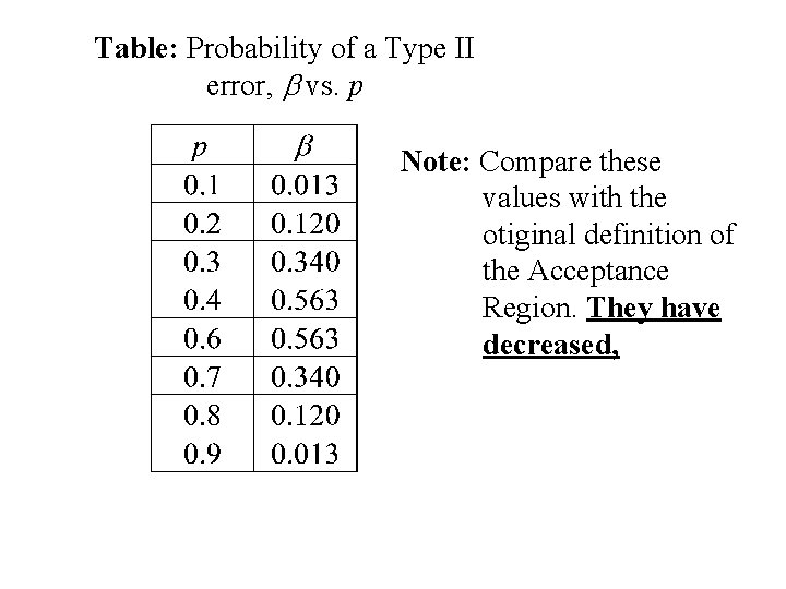
Table: Probability of a Type II error, b vs. p Note: Compare these values with the otiginal definition of the Acceptance Region. They have decreased,

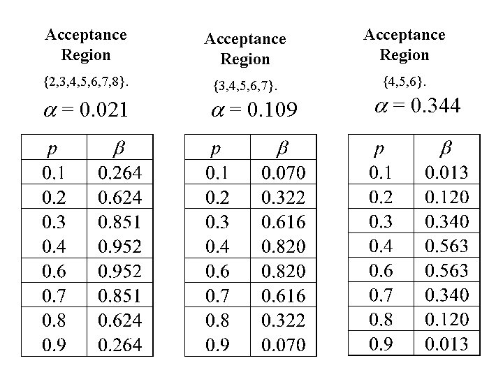
Acceptance Region {2, 3, 4, 5, 6, 7, 8}. {3, 4, 5, 6, 7}. {4, 5, 6}. a = 0. 021 a = 0. 109 a = 0. 344

The Approach in Statistical Testing is: • Set up the Acceptance Region so that a is close to some predetermine value (the usual values are 0. 05 or 0. 01) • The predetermine value of a (0. 05 or 0. 01) is called the significance level of the test. • The significance level of the test is a = P[test makes a type I error]

The z-test for Proportions Testing the probability of success in a binomial experiment

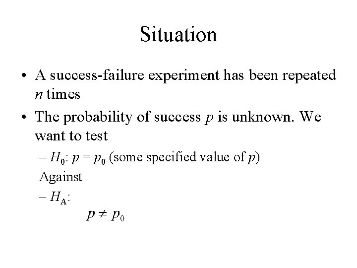
Situation • A success-failure experiment has been repeated n times • The probability of success p is unknown. We want to test – H 0: p = p 0 (some specified value of p) Against – H A:

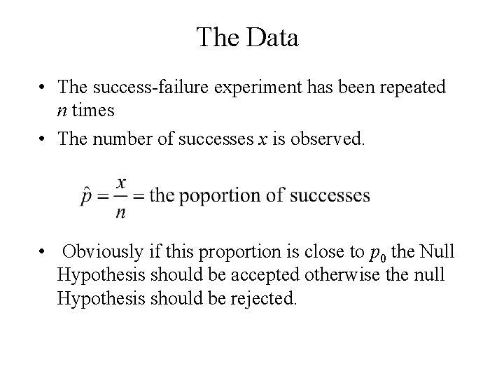
The Data • The success-failure experiment has been repeated n times • The number of successes x is observed. • Obviously if this proportion is close to p 0 the Null Hypothesis should be accepted otherwise the null Hypothesis should be rejected.

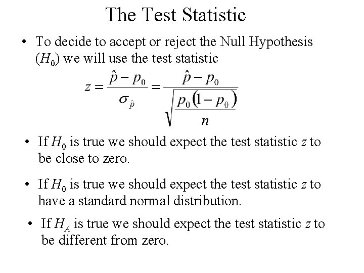
The Test Statistic • To decide to accept or reject the Null Hypothesis (H 0) we will use the test statistic • If H 0 is true we should expect the test statistic z to be close to zero. • If H 0 is true we should expect the test statistic z to have a standard normal distribution. • If HA is true we should expect the test statistic z to be different from zero.

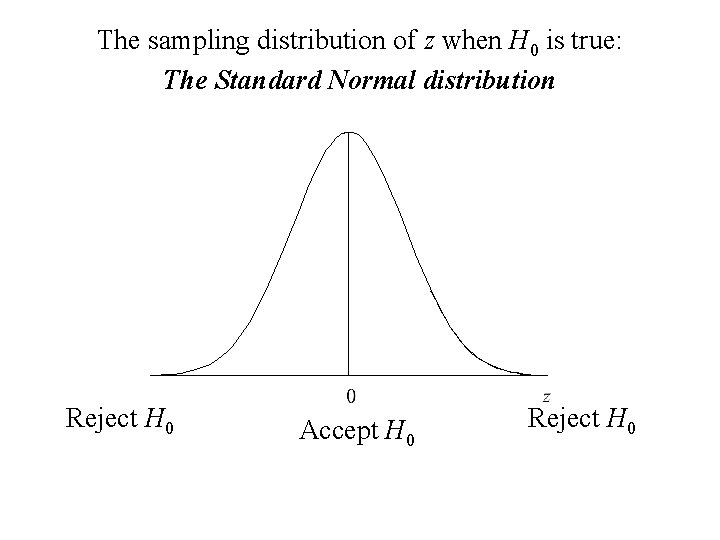
The sampling distribution of z when H 0 is true: The Standard Normal distribution Reject H 0 Accept H 0 Reject H 0

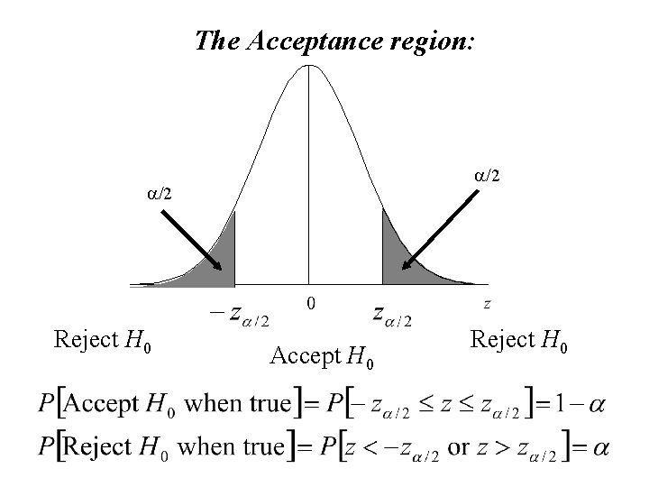
The Acceptance region: a/2 Reject H 0 Accept H 0 Reject H 0

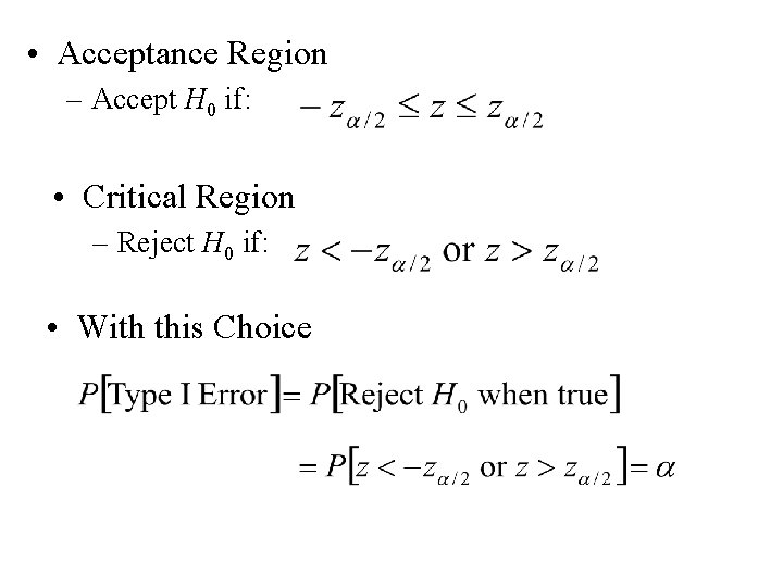
• Acceptance Region – Accept H 0 if: • Critical Region – Reject H 0 if: • With this Choice

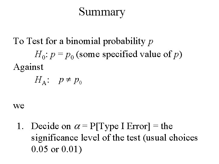
Summary To Test for a binomial probability p H 0: p = p 0 (some specified value of p) Against H A: we 1. Decide on a = P[Type I Error] = the significance level of the test (usual choices 0. 05 or 0. 01)

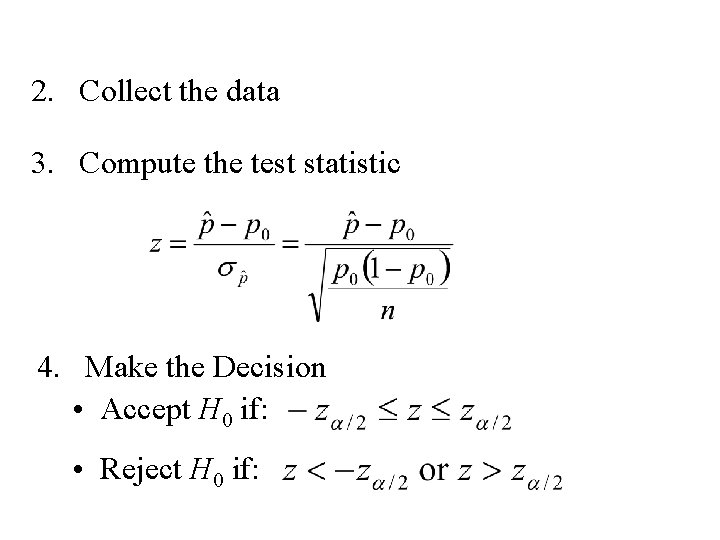
2. Collect the data 3. Compute the test statistic 4. Make the Decision • Accept H 0 if: • Reject H 0 if:

Example • In the last election the proportion of the voters who voted for the Liberal party was 0. 08 (8 %) • The party is interested in determining if that percentage has changed • A sample of n = 800 voters are surveyed

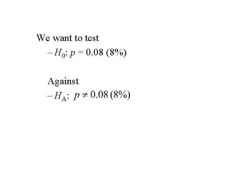
We want to test – H 0: p = 0. 08 (8%) Against – H A:

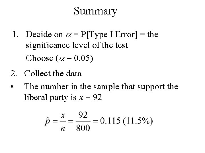
Summary 1. Decide on a = P[Type I Error] = the significance level of the test Choose (a = 0. 05) 2. Collect the data • The number in the sample that support the liberal party is x = 92

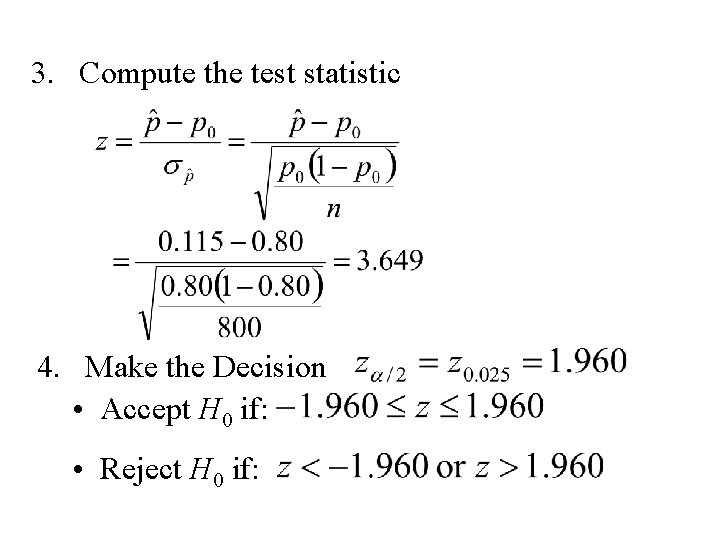
3. Compute the test statistic 4. Make the Decision • Accept H 0 if: • Reject H 0 if:

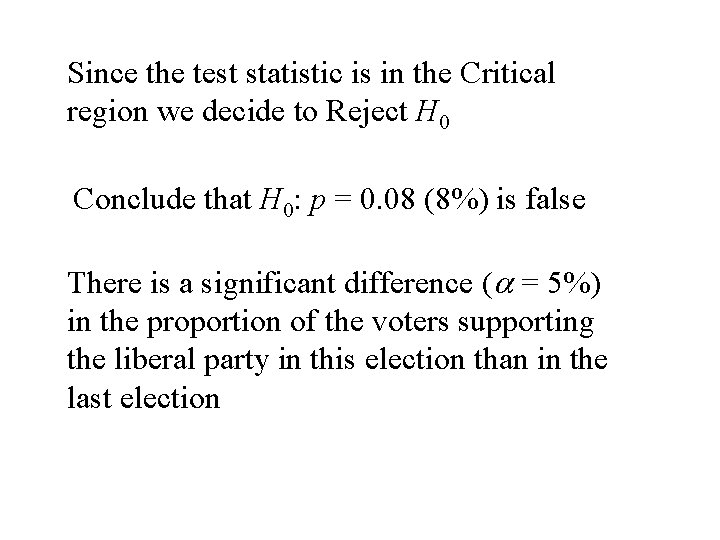
Since the test statistic is in the Critical region we decide to Reject H 0 Conclude that H 0: p = 0. 08 (8%) is false There is a significant difference (a = 5%) in the proportion of the voters supporting the liberal party in this election than in the last election

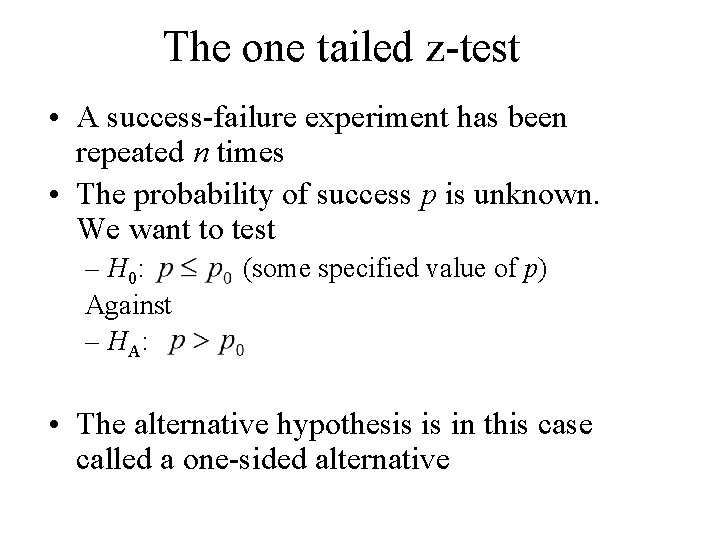
The one tailed z-test • A success-failure experiment has been repeated n times • The probability of success p is unknown. We want to test – H 0: Against – H A: (some specified value of p) • The alternative hypothesis is in this case called a one-sided alternative

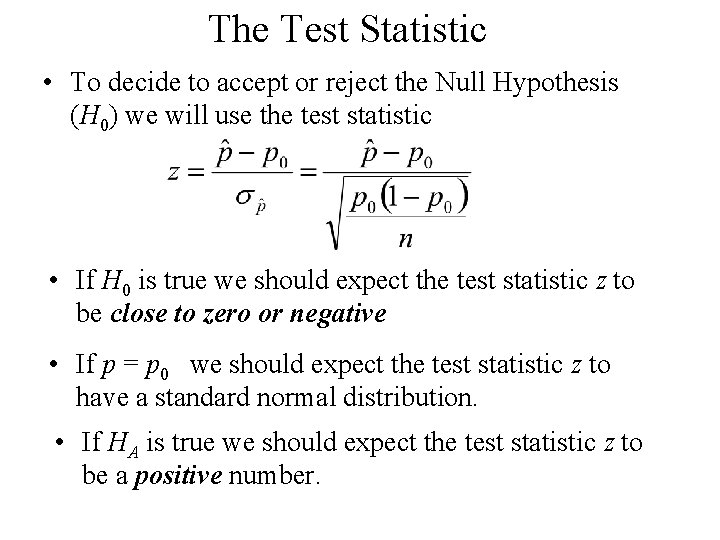
The Test Statistic • To decide to accept or reject the Null Hypothesis (H 0) we will use the test statistic • If H 0 is true we should expect the test statistic z to be close to zero or negative • If p = p 0 we should expect the test statistic z to have a standard normal distribution. • If HA is true we should expect the test statistic z to be a positive number.

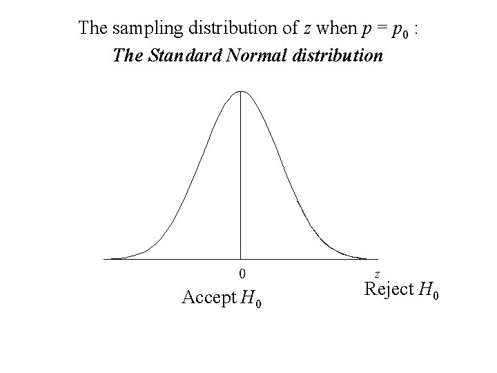
The sampling distribution of z when p = p 0 : The Standard Normal distribution Accept H 0 Reject H 0

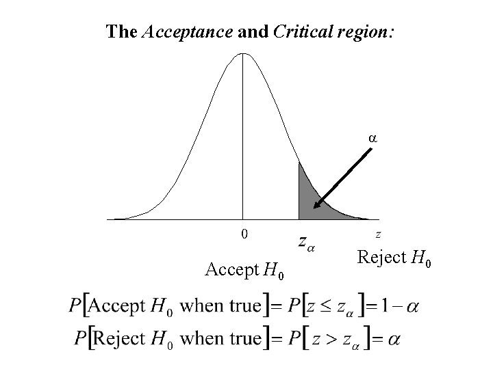
The Acceptance and Critical region: a Accept H 0 Reject H 0

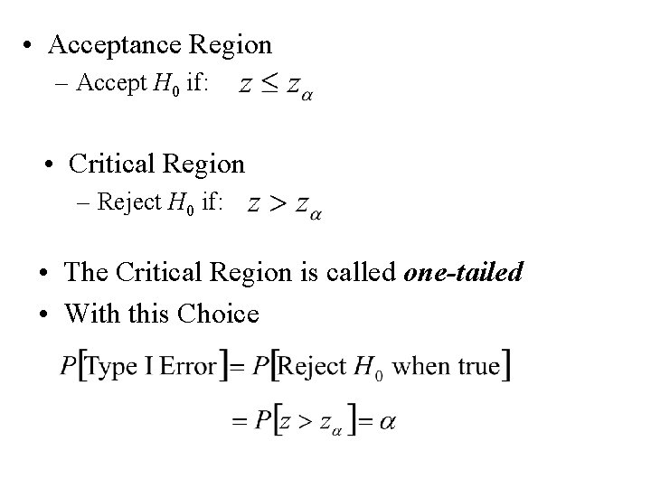
• Acceptance Region – Accept H 0 if: • Critical Region – Reject H 0 if: • The Critical Region is called one-tailed • With this Choice

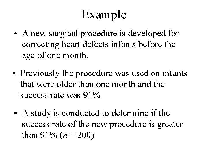
Example • A new surgical procedure is developed for correcting heart defects infants before the age of one month. • Previously the procedure was used on infants that were older than one month and the success rate was 91% • A study is conducted to determine if the success rate of the new procedure is greater than 91% (n = 200)

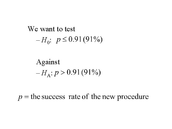
We want to test – H 0: Against – H A:

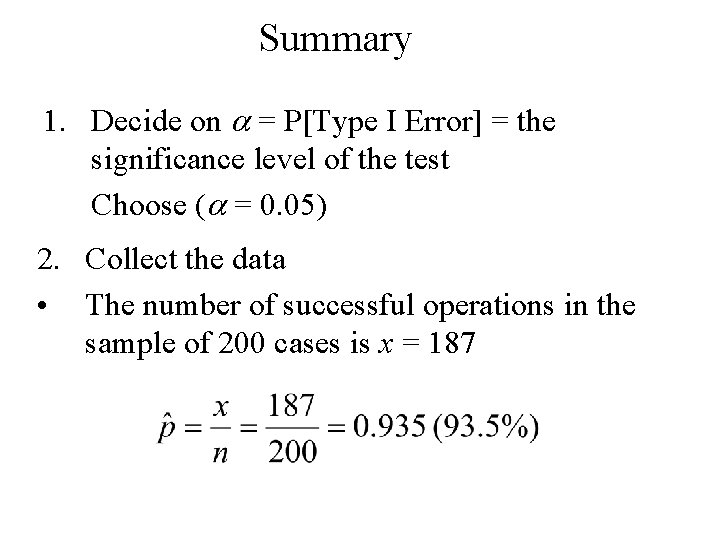
Summary 1. Decide on a = P[Type I Error] = the significance level of the test Choose (a = 0. 05) 2. Collect the data • The number of successful operations in the sample of 200 cases is x = 187

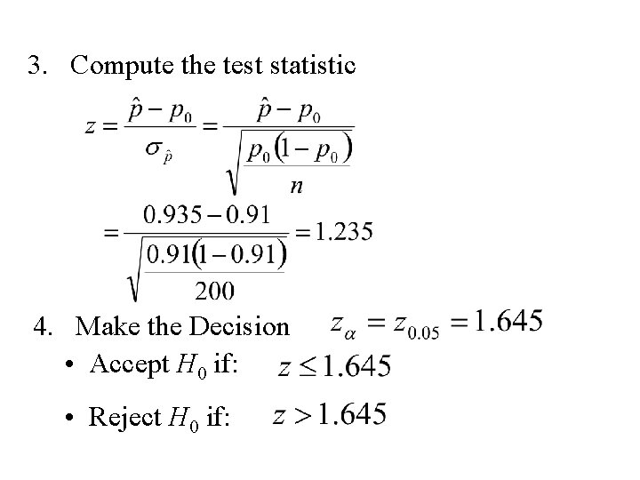
3. Compute the test statistic 4. Make the Decision • Accept H 0 if: • Reject H 0 if:

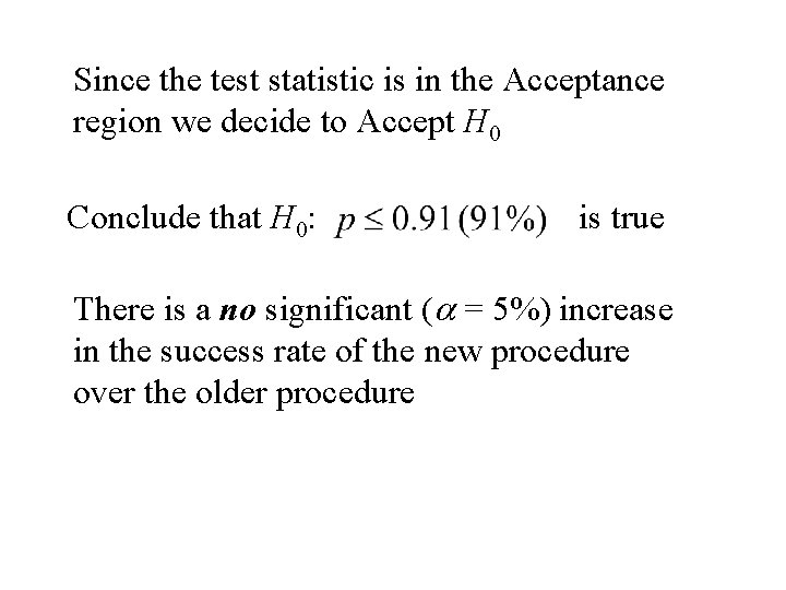
Since the test statistic is in the Acceptance region we decide to Accept H 0 Conclude that H 0: is true There is a no significant (a = 5%) increase in the success rate of the new procedure over the older procedure

Comments • When the decision is made to accept H 0 is made it should not be conclude that we have proven H 0. • This is because when setting up the test we have not controlled b = P[type II error] = P[accepting H 0 when H 0 is FALSE] • Whenever H 0 is accepted there is a possibility that a type II error has been made.

In the last example The conclusion that there is a no significant (a = 5%) increase in the success rate of the new procedure over the older procedure should be interpreted: We have been unable to proof that the new procedure is better than the old procedure

An analogy – a jury trial The two possible decisions are – Declare the accused innocent. – Declare the accused guilty.

The null hypothesis (H 0) – the accused is innocent The alternative hypothesis (HA) – the accused is guilty

The two possible errors that can be made: – Declaring an innocent person guilty. (type I error) – Declaring a guilty person innocent. (type II error) Note: in this case one type of error may be considered more serious

Requiring all 12 jurors to support a guilty verdict : – Ensures that the probability of a type I error (Declaring an innocent person guilty) is small. – However the probability of a type II error (Declaring an guilty person innocent) could be large.

Hence: When decision of innocence is made: – It is not concluded that innocence has been proven but that – we have been unable to disprove innocence

The z-test for the Mean of a Normal Population We want to test, m, denote the mean of a normal population

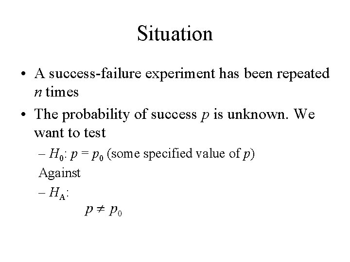
Situation • A success-failure experiment has been repeated n times • The probability of success p is unknown. We want to test – H 0: p = p 0 (some specified value of p) Against – H A:

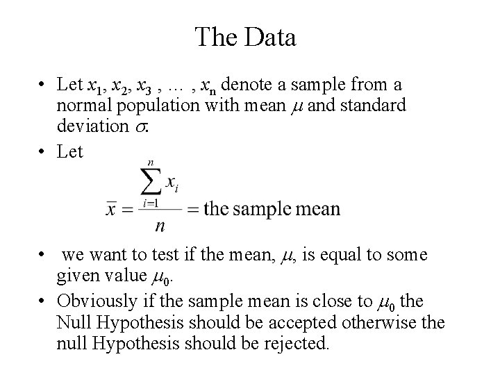
The Data • Let x 1, x 2, x 3 , … , xn denote a sample from a normal population with mean m and standard deviation s. • Let • we want to test if the mean, m, is equal to some given value m 0. • Obviously if the sample mean is close to m 0 the Null Hypothesis should be accepted otherwise the null Hypothesis should be rejected.

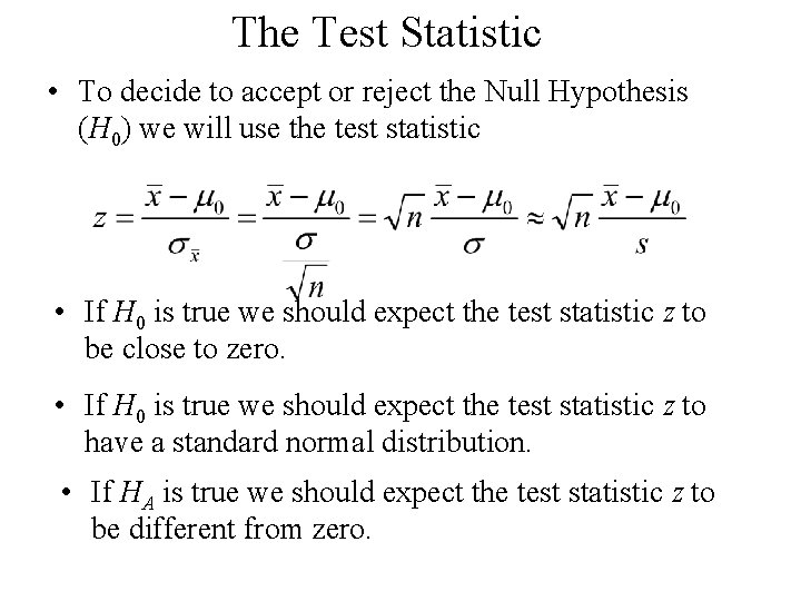
The Test Statistic • To decide to accept or reject the Null Hypothesis (H 0) we will use the test statistic • If H 0 is true we should expect the test statistic z to be close to zero. • If H 0 is true we should expect the test statistic z to have a standard normal distribution. • If HA is true we should expect the test statistic z to be different from zero.

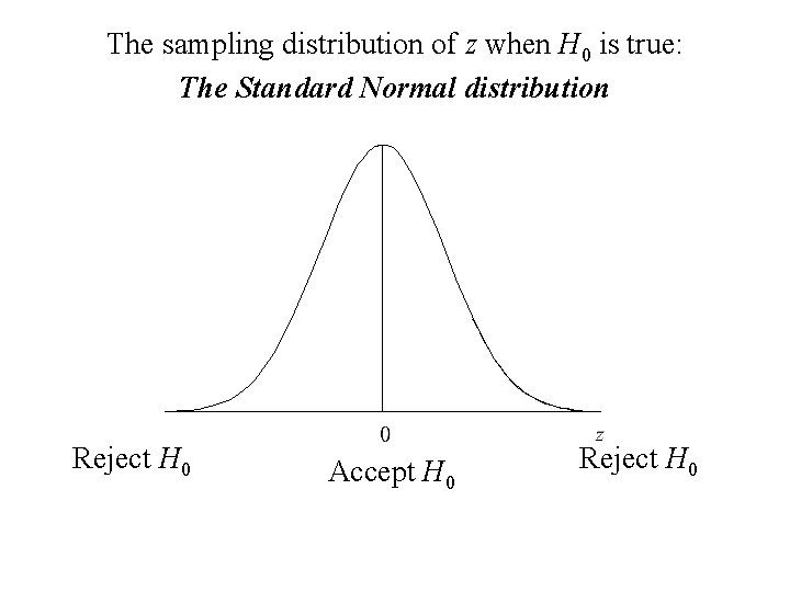
The sampling distribution of z when H 0 is true: The Standard Normal distribution Reject H 0 Accept H 0 Reject H 0

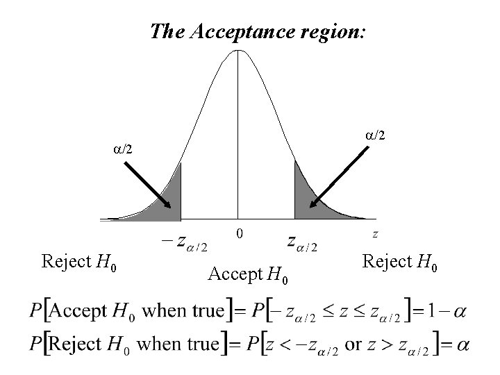
The Acceptance region: a/2 Reject H 0 Accept H 0 Reject H 0

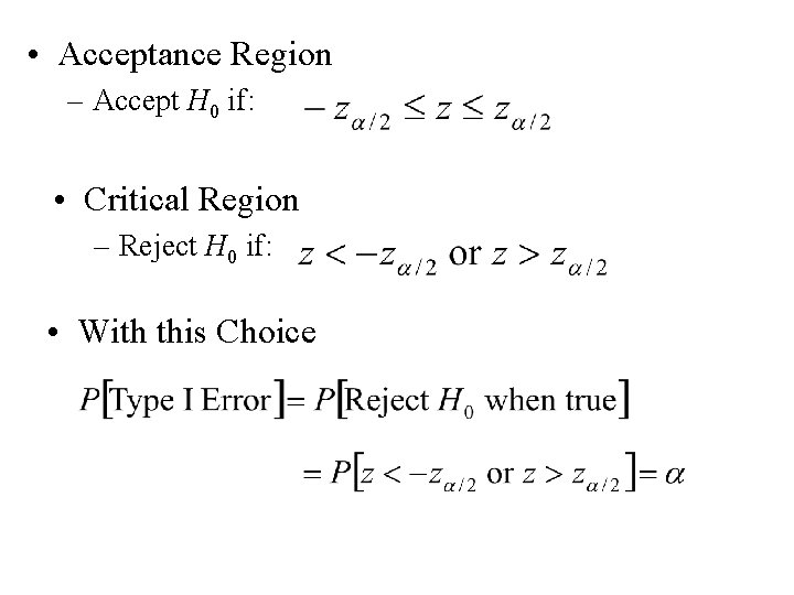
• Acceptance Region – Accept H 0 if: • Critical Region – Reject H 0 if: • With this Choice

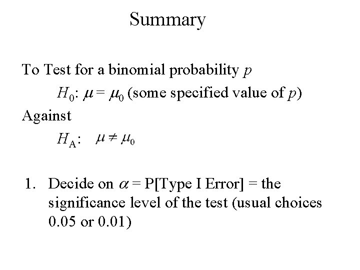
Summary To Test for a binomial probability p H 0: m = m 0 (some specified value of p) Against H A: 1. Decide on a = P[Type I Error] = the significance level of the test (usual choices 0. 05 or 0. 01)

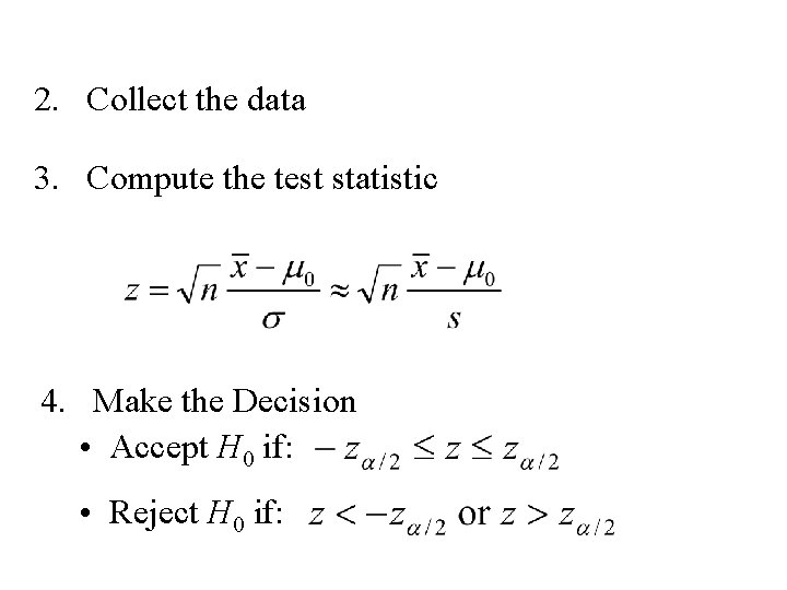
2. Collect the data 3. Compute the test statistic 4. Make the Decision • Accept H 0 if: • Reject H 0 if:

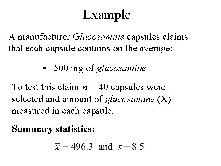
Example A manufacturer Glucosamine capsules claims that each capsule contains on the average: • 500 mg of glucosamine To test this claim n = 40 capsules were selected and amount of glucosamine (X) measured in each capsule. Summary statistics:

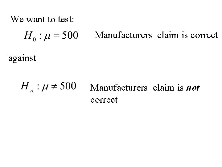
We want to test: Manufacturers claim is correct against Manufacturers claim is not correct

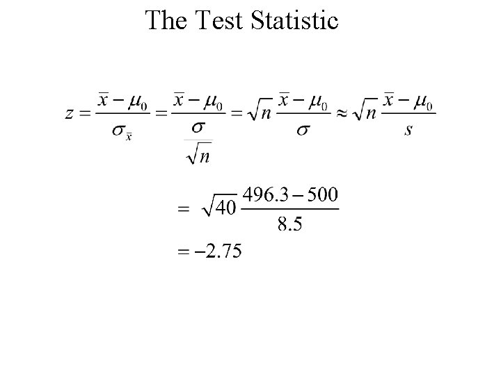
The Test Statistic

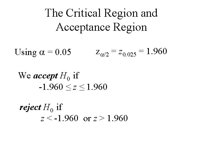
The Critical Region and Acceptance Region Using a = 0. 05 za/2 = z 0. 025 = 1. 960 We accept H 0 if -1. 960 ≤ z ≤ 1. 960 reject H 0 if z < -1. 960 or z > 1. 960

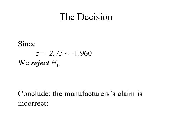
The Decision Since z= -2. 75 < -1. 960 We reject H 0 Conclude: the manufacturers’s claim is incorrect: