Statistical Inference Correlation Simple Linear Regression April 17


 is")

 abline(lm(y ~")


 function • The first argument of the lm() function is")


: P-value for the above F test.")


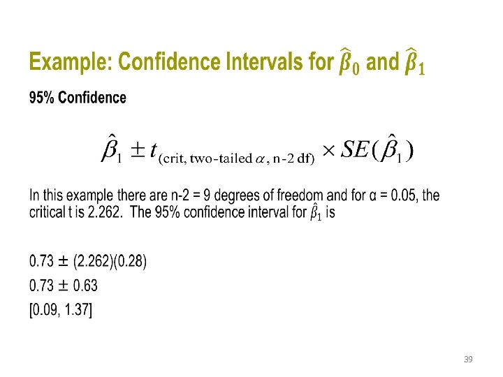
 • confint(model 1) 38")


, and age (years),")


- Slides: 47
Statistical Inference Correlation & Simple Linear Regression April 17, 2018
Correlation analysis* • Measuring the degree of association between two continuous variables, x and y • We have a linear relationship between x and y if a straight line drawn through the midst of the points provides the most appropriate approximation to the observed relationship • We measure how close the observations are to the straight line that best describes their linear relationship by calculating the Pearson product moment correlation coefficient, usually simply called the correlation coefficient *The following slides were adapted from Prof. Trinquart’s R Course (BS 730) 2
Example 3
Pearson product moment correlation coefficient estimate of the population correlation coefficient, ρ 4
Pearson product moment correlation coefficient • between -1 and +1 • indicates the direction and strength of the linear relationship – r>0 one variable increases as the other variable increases – r<0: one variable decreases as the other increases – r = 0 : no linear correlation (although there may be a nonlinear relationship) – r = +1 or -1: perfect linear correlation with all the points lying on the line – the closer r is to the extremes, the greater the degree of linear association 5
Rule of thumb • • • r≥ 0. 9 very highly correlated variables (r 2 ≥ 81%) 0. 7≤r<0. 9 highly correlated (49% ≤ r 2 < 81%) 0. 5≤r<0. 7 moderately correlated (25% ≤ r 2 < 49%) 0. 3≤r< 0. 5 low correlation (9% ≤ r 2 < 25%) r<0. 3 little if any (linear) correlation ( r 2 < 9%) 6
Pearson product moment correlation coefficient • valid only within the range of values of x and y in the sample • x and y can be interchanged without affecting the value of r • (linear) correlation does not imply a cause/effect relationship • r 2 proportion of variability in y that can be explained by its linear relationship with x (coefficient of determination) 7
When not to calculate Pearson’s r • when there is a non-linear relationship (eg Ushaped and J-shaped relationships) • when there are outliers • when there are subgroups for which the mean of least one of the variables are different 8
Pearson Correlation Assumptions • Observations are independent • The association is linear • Variables are approximately normally distributed 9
Statistical significance ≠ Clinical relevance • The significance of a given correlation coefficient is a function of sample size; i. e. , a low correlation can be significant if the sample size is large enough 10
Hypothesis Testing • H 0: There is no correlation between the two variables ρ=0 • H 1: There is a correlation between the two variables ρ≠ 0 11
Pearson correlation test statistic • The Student’s t distribution is used where se(r) is defined as • Note that the standard error is inversely related to n. A larger sample size corresponds to a smaller se(r). • If the population correlation is zero and assuming x and y follow normal distributions, then the test statistic has a Student’s t distribution with n-2 degrees of freedom 12
Confidence Interval for ρ • Since r is an estimate of a parameter, we can calculate a confidence interval for the population correlation coefficient, ρ • Based on z = 0. 5 ln[(1+r)/(1 -r)] • Because the transformation is a non-linear function of r, the confidence interval is not symmetric around r. 13
In R • Begin with a scatter plot! plot(x, y, xlab="x-label", ylab="y-label") abline(lm(y ~ x)) cor( x, y, method = “pearson") cor. test(x, y, method=“pearson") • default method is "pearson" so you may omit the method option 14
Example 15
Example: Reporting Results H 0: There is no linear association between age and SBP (ρ=0) H 1: There is a linear association between age and SBP (ρ≠ 0) Pearson’s correlation was used to determine if there was a linear association between age and systolic blood pressure (SBP) There is significant evidence at α=0. 05 of a moderate, positive, linear association between age and SBP, r = 0. 65 with a 95% C. I. of 0. 09 to 0. 90, p-value = 0. 029. 16
Simple Linear Regression
Background • Even as more and more sophisticated statistical procedures are developed, linear regression remains a fundamental element of the quantitative health sciences. • Concept of regression and correlation invented by Francis Galton (b. 1822; d. 1911) • Studied relationship between parental and child height • Contemporary paper in European Journal of Human Genetics showed that modern methods improved little on the original predictive model. Source: Predicting Height: The Victorian Approach Beats Modern Genomics http: //www. wired. com/2009/03/predicting-height-the-victorian-approach-beats-modern-genomics/
Modern Example from Simply Statistics • “Data supports claim that if Kobe stops ball hogging the Lakers will win more” • “Linear regression suggests that an increase of 1% in % of shots taken by Kobe results in a drop of 1. 16 points (+/- 0. 22) in score differential. ” Source: http: //simplystatistics. org/2013/01/28/data-supports-claim-that-if-kobe-stops-ball-hogging-the-lakers-will-win-more/
Questions we might ask with linear regression • To use the parents' heights to predict child heights. • To try to find a parsimonious, easily described mean relationship between parent and children's heights. • To investigate the variation in child heights that appears unrelated to parents' heights (residual variation). • To quantify what impact genotype information has beyond parental height in explaining child height. • To figure out how/whether and what assumptions are needed to generalize findings beyond the data in question. • Why do children of very tall parents tend to be tall, but a little shorter than their parents and why children of very short parents tend to be short, but a little taller than their parents? (This is a famous question called 'Regression to the mean'. )
Linear Regression • If we believe y is dependent on x, with a change in y being attributed to a change in x, rather than the other way round, we can determine the linear regression line (the regression of y on x) that best describes the straight line relationship between the two variables 21
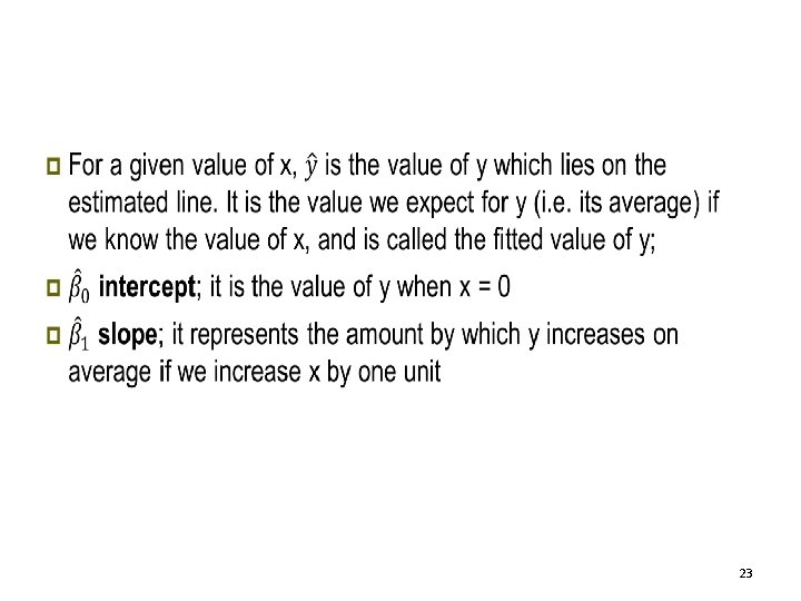
Model • Find the equation of the line that best fits the data. The generic equation of the line relating y to x is of the form: • In the sample, the equation of the line of “best fit” is written as: • NOTE: The actual data will NEVER fall exactly on this "best fit" line. That’s why the model contains an error term. The error term contains the influences of other factors not captured by the model. 22
Observed Residual Predicted 24
Method of least squares • The "best fit" line is the line that minimizes the sum of the squared residuals. • Want to minimize: • For linear regressions with only one independent variable, X, this yields the following equations: 25
Example: Model for SBP and Age • For the previous example using SBP and age: 26
Example: best fit and predicted value • The "best fit" line for these data is: • Predicted SBP for a person that is 24 years old: • There was an observed SBP value of 116 at age=24. The residual at age=24 is • The range of age in the given data was 22 - 40. Therefore, we should not use the above model to predict the SBP for a 65 yr old person 27
correlation and coefficient of simple linear regression • 28
In R • lm() function • The first argument of the lm() function is a formula object, with the outcome specified followed by the ~ operator then the predictors mod 1 <- lm(y ~ x, data=ds) summary(mod 1) summary. aov(mod 1) 29
Example: sbp and age 30
Example: ANOVA table Sum of Squares 31
Example: Sum of Squares • Model SS = SS of the differences between y predicted by the model and the overall average. • Error SS = SS of the differences between observed y and y predicted by the model. • Total SS = SS of the differences between observed y and the overall average. • The better the model fits, the larger the model SS is and the smaller the error SS 32
F test F value: test statistic for the overall model In a situation with only a single X variable, the F-test is equivalent to the t test for the null hypothesis that β 1=0 33
p-value of the goodness of the fit Pr(>F): P-value for the above F test. 34
R 2 • R 2 proportion of variability in y explained by the independent variable(s) • R 2 = (Model SS / Total SS) = 158. 93/(158. 93+213. 26) = 0. 427 • R-square takes values between 0 and 1 and measures the goodness of fit of the model. Values close to 1 are indicative of a good fit 35
R 2 • When there is only one independent variable, x, • R 2 is the proportion of the variability in y that can be explained by x. • R 2 is equal to the square of the Pearson correlation between x and y 36
Parameter estimates • 37
Confidence interval • model 1<-lm(sbp~age, data=ds) • confint(model 1) 38
Example: Testing of parameters Test for Prob > |t| are the p-values for the t-tests 40
Example: testing the parameter • 41
Example: Reporting Results • 42
Example: Reporting Results – Technical Summary • H 0: There is no linear association between SBP and age among women ages 22 -40. • H 1: There is a linear association between SBP and age among women ages 22 -40. • OR H 0: βage = 0 vs H 1: βage ≠ 0 43
Example: Reporting Results – Technical Summary Conclusion of hypothesis test: Reject H 0. There is significant evidence at α=0. 05 of a linear association between SBP and age among women ages 22 -40 (t=2. 59, df=9). 44
Sample Write-up Methods To examine the association between SBP (mm. Hg), and age (years), we performed a linear regression analysis. We used a 0. 05 level of significance Results In the linear regression analysis of the association of SBP and age, we found that there was a significant, positive linear association, with an estimated slope of 0. 73 (t=2. 59, df=9; p = 0. 0292). On average, a one year increase in age corresponds to an increase of 0. 73 mm. Hg in SBP. The R 2 for this model was 0. 43 (age accounts for 43% of the variability of SBP in these data). 45
Express results for a continuous independent variable • 46
Deliverables • Due 4/22 – Complete draft • Due 4/29 – Final Research Paper • Due 5/8 – Final presentation