Statistical Genomics Lecture 20 MLMM Zhiwu Zhang Washington

Statistical Genomics Lecture 20: MLMM Zhiwu Zhang Washington State University

Administration Homework 4 graded Homework 5, due April 13, Wednesday, 3: 10 PM Final exam: May 3, 120 minutes (3: 10 -5: 10 PM), 50 Department seminar (March 28) , Brigid Meints, “Breeding Barley and Beans for Western Washington”

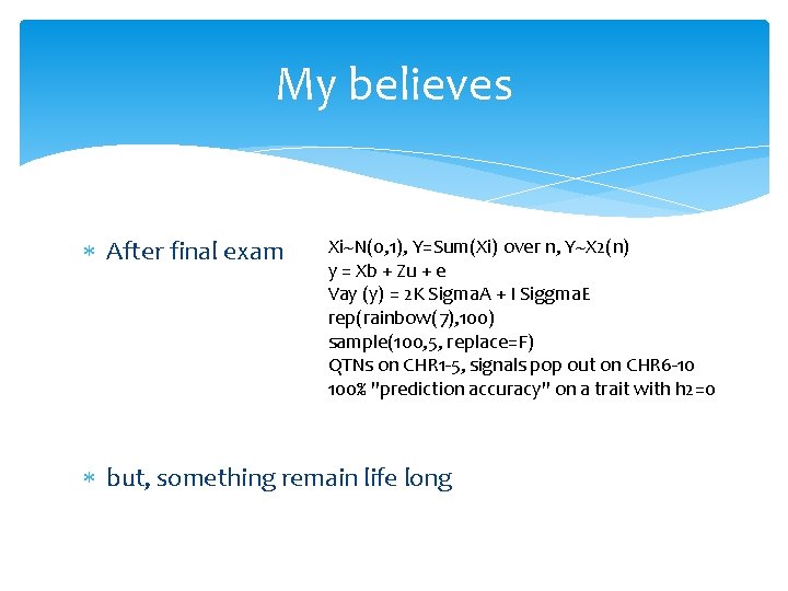
My believes After final exam Xi~N(0, 1), Y=Sum(Xi) over n, Y~X 2(n) y = Xb + Zu + e Vay (y) = 2 K Sigma. A + I Siggma. E rep(rainbow(7), 100) sample(100, 5, replace=F) QTNs on CHR 1 -5, signals pop out on CHR 6 -10 100% "prediction accuracy" on a trait with h 2=0 but, something remain life long

Core values behind statistics, programming, genetics, GWAS and GS in CROPS 545 Doing >> looking Reasoning Learn = (re)invent Creative Self confidence

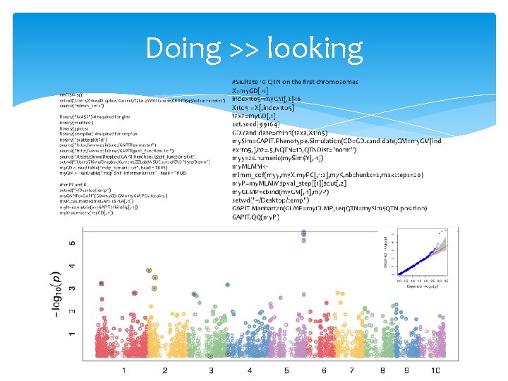
Doing >> looking

Reasoning Teaching model Hypothesis: There is no space to improve Objective: Reject the null hypothesis Method: Increase statistical power

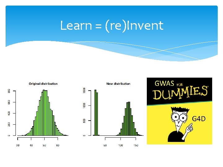
Learn = (re)Invent

Creative Dare to break the rules with judgment

Self confidence Questioning why decreasing missing rate does not improve accuracy of stochastic imputation by Chongqing Questioning what is "u" in MLM by Joe Finding of setting seed in impute (KNN) package by Louisa One more example of my own

Evaluation Comment: Much more work than other WSU courses Adjustment 1. Assignments: 9 to 6 2. Requirements: No experience with statistics and programming 3. Easy to pass, or a grade C- after 1 st assignment unless unusual behavior or recommended to withdraw

Outline Stepwise regression Criteria MLMM Power vs FDR and Type I error Replicate and mean

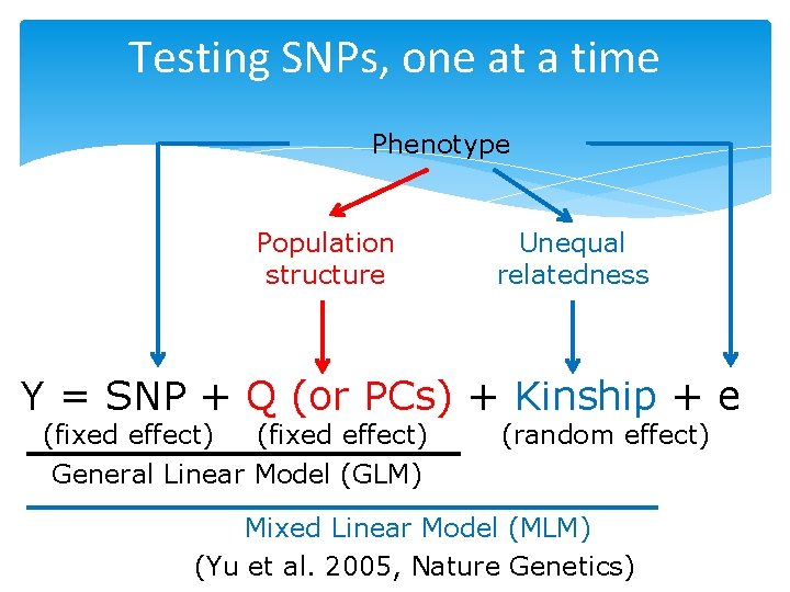
Testing SNPs, one at a time Phenotype Population structure Unequal relatedness Y = SNP + Q (or PCs) + Kinship + e (fixed effect) General Linear Model (GLM) (random effect) Mixed Linear Model (MLM) (Yu et al. 2005, Nature Genetics)

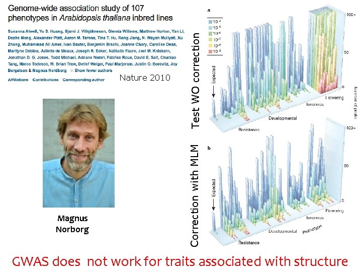
Magnus Norborg Test WO correction Correction with MLM Nature 2010 GWAS does not work for traits associated with structure

Two years later

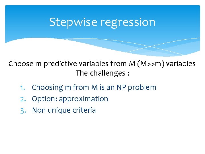
Stepwise regression Choose m predictive variables from M (M>>m) variables The challenges : 1. Choosing m from M is an NP problem 2. Option: approximation 3. Non unique criteria

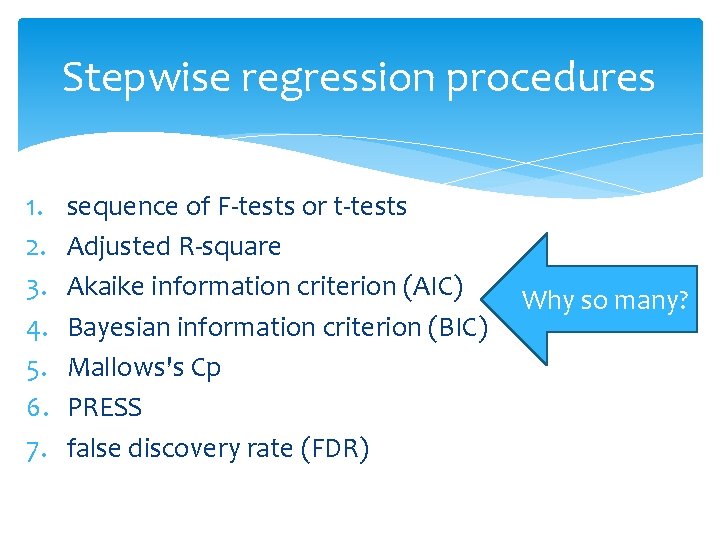
Stepwise regression procedures 1. 2. 3. 4. 5. 6. 7. sequence of F-tests or t-tests Adjusted R-square Akaike information criterion (AIC) Bayesian information criterion (BIC) Mallows's Cp PRESS false discovery rate (FDR) Why so many?

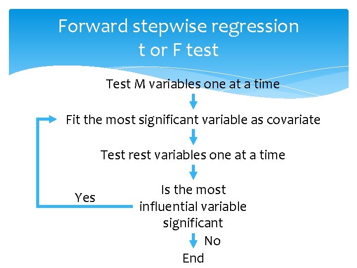
Forward stepwise regression t or F test Test M variables one at a time Fit the most significant variable as covariate Test rest variables one at a time Yes Is the most influential variable significant No End

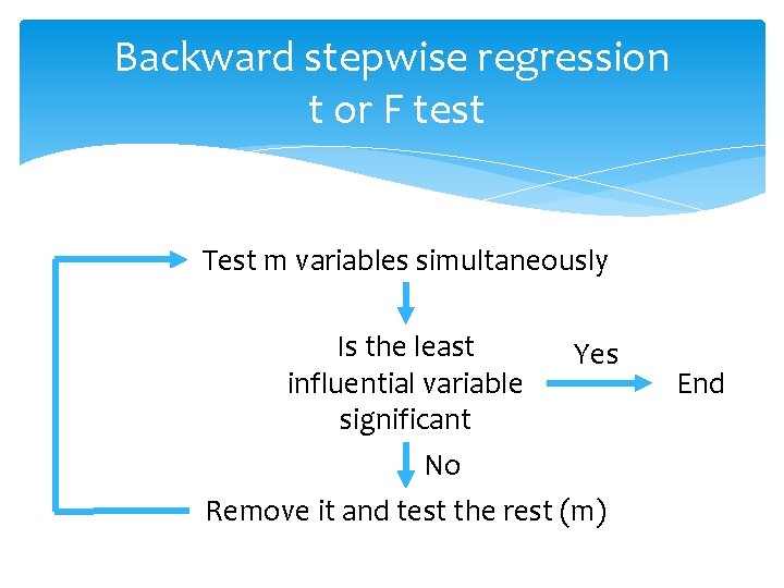
Backward stepwise regression t or F test Test m variables simultaneously Is the least Yes influential variable significant No Remove it and test the rest (m) End

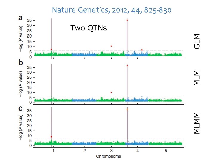
Hind from MHC (Major histocompatibility complex)

Nature Genetics, 2012, 44, 825 -830 MLMM MLM GLM Two QTNs

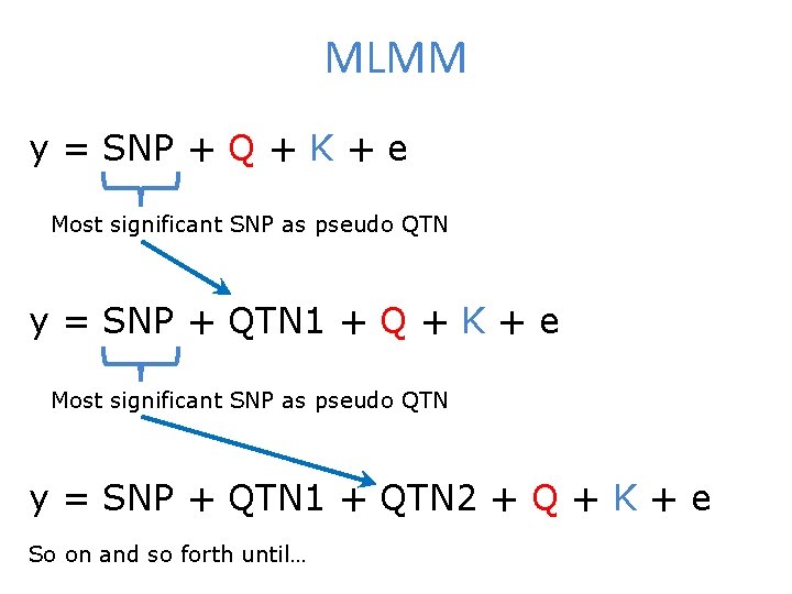
MLMM y = SNP + Q + K + e Most significant SNP as pseudo QTN y = SNP + QTN 1 + QTN 2 + Q + K + e So on and so forth until…

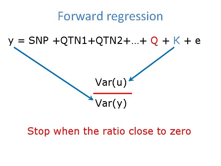
Forward regression y = SNP +QTN 1+QTN 2+…+ Q + K + e Var(u) Var(y) Stop when the ratio close to zero

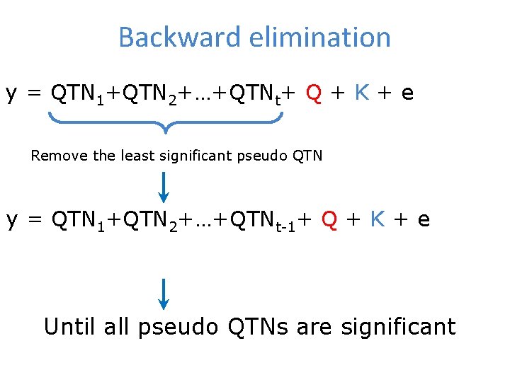
Backward elimination y = QTN 1+QTN 2+…+QTNt+ Q + K + e Remove the least significant pseudo QTN y = QTN 1+QTN 2+…+QTNt-1+ Q + K + e Until all pseudo QTNs are significant

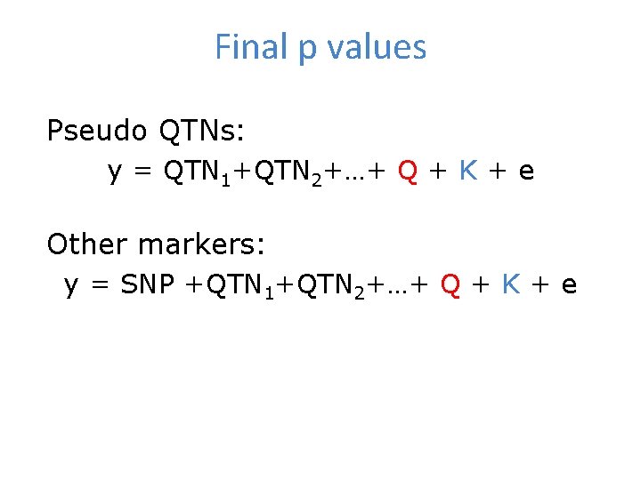
Final p values Pseudo QTNs: y = QTN 1+QTN 2+…+ Q + K + e Other markers: y = SNP +QTN 1+QTN 2+…+ Q + K + e

MLMM R on Git. Hub

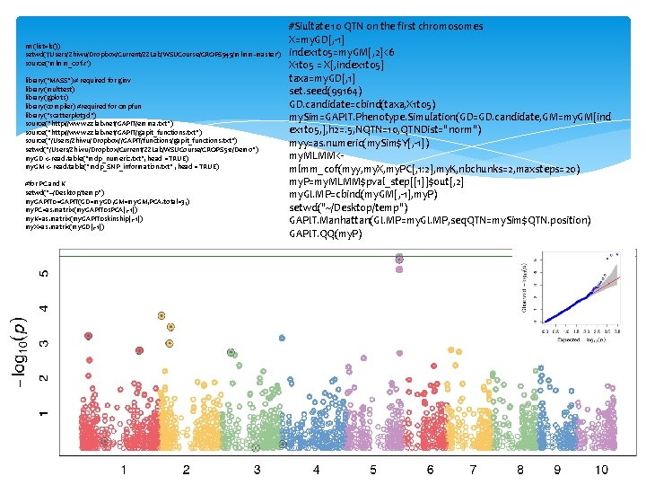
rm(list=ls()) setwd('/Users/Zhiwu/Dropbox/Current/ZZLab/WSUCourse/CROPS 545/mlmm-master') source('mlmm_cof. r') library("MASS") # required for ginv library(multtest) library(gplots) library(compiler) #required for cmpfun library("scatterplot 3 d") source("http: //www. zzlab. net/GAPIT/emma. txt") source("http: //www. zzlab. net/GAPIT/gapit_functions. txt") source("/Users/Zhiwu/Dropbox//GAPIT/functions/gapit_functions. txt") setwd("/Users/Zhiwu/Dropbox/Current/ZZLab/WSUCourse/CROPS 512/Demo") my. GD <- read. table("mdp_numeric. txt", head = TRUE) my. GM <- read. table("mdp_SNP_information. txt" , head = TRUE) #for PC and K setwd("~/Desktop/temp") my. GAPIT 0=GAPIT(GD=my. GD, GM=my. GM, PCA. total=3, ) my. PC=as. matrix(my. GAPIT 0$PCA[, -1]) my. K=as. matrix(my. GAPIT 0$kinship[, -1]) my. X=as. matrix(my. GD[, -1]) #Siultate 10 QTN on the first chromosomes X=my. GD[, -1] index 1 to 5=my. GM[, 2]<6 X 1 to 5 = X[, index 1 to 5] taxa=my. GD[, 1] set. seed(99164) GD. candidate=cbind(taxa, X 1 to 5) my. Sim=GAPIT. Phenotype. Simulation(GD=GD. candidate, GM=my. GM[ind ex 1 to 5, ], h 2=. 5, NQTN=10, QTNDist="norm") myy=as. numeric(my. Sim$Y[, -1]) my. MLMM<mlmm_cof(myy, my. X, my. PC[, 1: 2], my. K, nbchunks=2, maxsteps=20) my. P=my. MLMM$pval_step[[1]]$out[, 2] my. GI. MP=cbind(my. GM[, -1], my. P) setwd("~/Desktop/temp") GAPIT. Manhattan(GI. MP=my. GI. MP, seq. QTN=my. Sim$QTN. position) GAPIT. QQ(my. P)

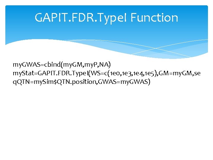
GAPIT. FDR. Type. I Function my. GWAS=cbind(my. GM, my. P, NA) my. Stat=GAPIT. FDR. Type. I(WS=c(1 e 0, 1 e 3, 1 e 4, 1 e 5), GM=my. GM, se q. QTN=my. Sim$QTN. position, GWAS=my. GWAS)

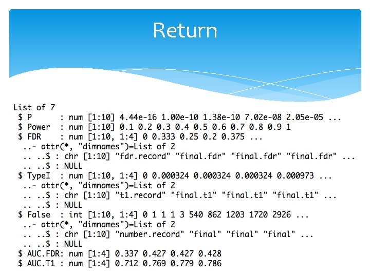
Return

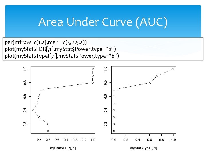
Area Under Curve (AUC) par(mfrow=c(1, 2), mar = c(5, 2, 5, 2)) plot(my. Stat$FDR[, 1], my. Stat$Power, type="b") plot(my. Stat$Type. I[, 1], my. Stat$Power, type="b")

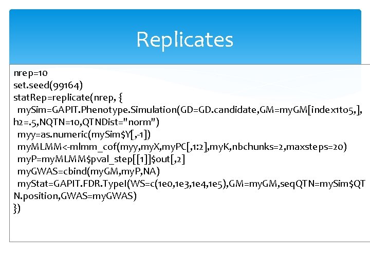
Replicates nrep=10 set. seed(99164) stat. Rep=replicate(nrep, { my. Sim=GAPIT. Phenotype. Simulation(GD=GD. candidate, GM=my. GM[index 1 to 5, ], h 2=. 5, NQTN=10, QTNDist="norm") myy=as. numeric(my. Sim$Y[, -1]) my. MLMM<-mlmm_cof(myy, my. X, my. PC[, 1: 2], my. K, nbchunks=2, maxsteps=20) my. P=my. MLMM$pval_step[[1]]$out[, 2] my. GWAS=cbind(my. GM, my. P, NA) my. Stat=GAPIT. FDR. Type. I(WS=c(1 e 0, 1 e 3, 1 e 4, 1 e 5), GM=my. GM, seq. QTN=my. Sim$QT N. position, GWAS=my. GWAS) })

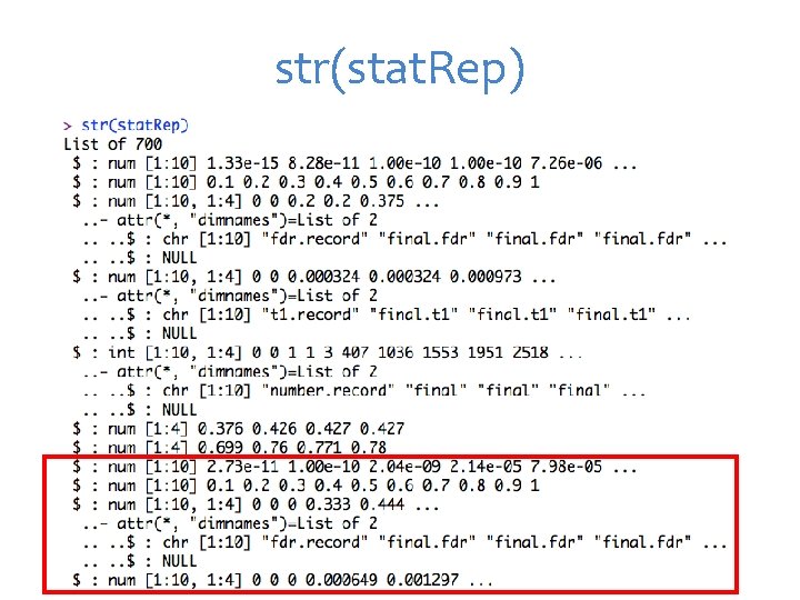
str(stat. Rep)

Means over replicates power=stat. Rep[[2]] #FDR s. fdr=seq(3, length(stat. Rep), 7) fdr=stat. Rep[s. fdr] fdr. mean=Reduce ("+", fdr) / length(fdr) #AUC: power vs. FDR s. auc. fdr=seq(6, length(stat. Rep), 7) auc. fdr=stat. Rep[s. auc. fdr] auc. fdr. mean=Reduce ("+", auc. fdr) / length(auc. fdr)

Plots of power vs. FDR the. Color=rainbow(4) plot(fdr. mean[, 1], power , type="b", col=the. Color [1], xlim=c(0, 1)) for(i in 2: ncol(fdr. mean)){ lines(fdr. mean[, i], power , type="b", col= the. Color [i]) }

Highlight Stepwise regression Criteria MLMM Power vs FDR and Type I error Replicate and mean