Statistical Disclosure Limitation Releasing Useful Data for Statistical

Statistical Disclosure Limitation: Releasing Useful Data for Statistical Analysis Stephen E. Fienberg Department of Statistics Center for Automated Learning & Discovery Center for Computer & Communications Security Carnegie Mellon University Pittsburgh, PA, U. S. A. BTS Confidentiality Seminar Series, April 2003 1

Restricted Access vs. Releasing Restricted Data • Restricted Access: – – – Special Sworn Employees. Licensed Researchers. External Sites. Firewalls. Query Control. • Releasing Restricted Data: – Confidentiality motivates possible transformation of data before release. – Assess risk of disclosure and harm. 2

Statistical Disclosure Limitation • What is goal of disclosure limitation? – “Protecting" confidentiality. – Providing access to statistical data: • Statistical users want more than to retrieve a few numbers. • They want data useful for statistical analysis. • Statistical disclosure limitation needs to assess tradeoff between preserving confidentiality and usefulness of released data, especially for inferential purposes. 3

What Makes Released Data Statistically Useful? • Inferences should be the same as if we had original data. – Reversing the disclosure protection mechanism, not for individual identification, but for inferences about parameters in statistical models (may require likelihood function for disclosure procedure). • Sufficient variables to allow for proper multivariate analyses. • Ability to assess goodness of fit of models. 4

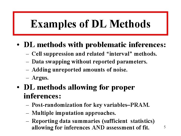
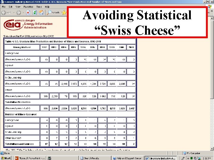
Examples of DL Methods • DL methods with problematic inferences: – – Cell suppression and related “interval” methods. Data swapping without reported parameters. Adding unreported amounts of noise. Argus. • DL methods allowing for proper inferences: – Post-randomization for key variables–PRAM. – Multiple imputation approaches. – Reporting data summaries (sufficient statistics) allowing for inferences AND assessment of fit. 5

Avoiding Statistical “Swiss Cheese” 6

7

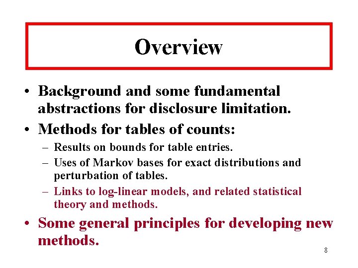
Overview • Background and some fundamental abstractions for disclosure limitation. • Methods for tables of counts: – Results on bounds for table entries. – Uses of Markov bases for exact distributions and perturbation of tables. – Links to log-linear models, and related statistical theory and methods. • Some general principles for developing new methods. 8

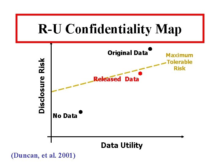
R-U Confidentiality Map Disclosure Risk Original Data Released Data No Data Utility (Duncan, et al. 2001) Maximum Tolerable Risk

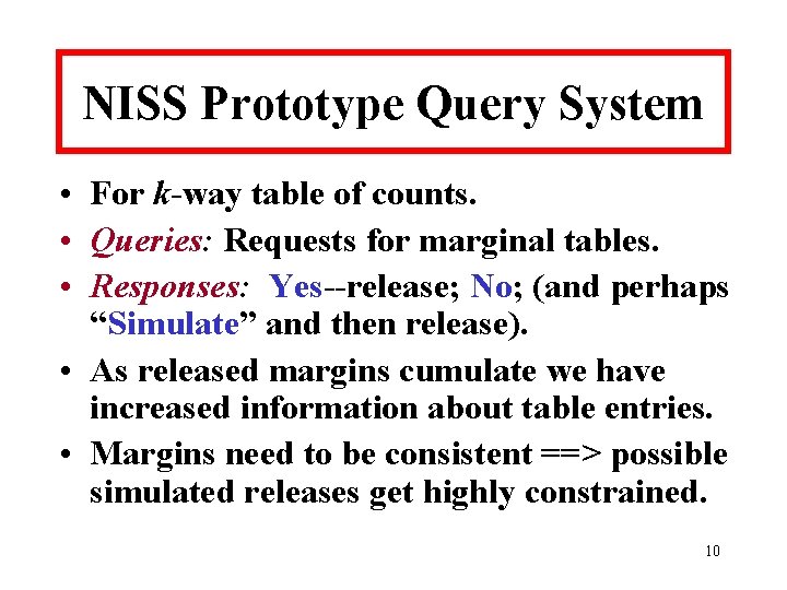
NISS Prototype Query System • For k-way table of counts. • Queries: Requests for marginal tables. • Responses: Yes--release; No; (and perhaps “Simulate” and then release). • As released margins cumulate we have increased information about table entries. • Margins need to be consistent ==> possible simulated releases get highly constrained. 10

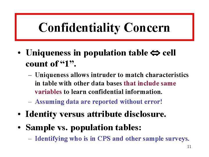
Confidentiality Concern • Uniqueness in population table cell count of “ 1”. – Uniqueness allows intruder to match characteristics in table with other data bases that include same variables to learn confidential information. – Assuming data are reported without error! • Identity versus attribute disclosure. • Sample vs. population tables: – Identifying who is in CPS and other sample surveys. 11

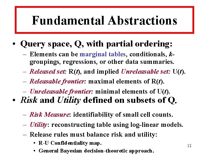
Fundamental Abstractions • Query space, Q, with partial ordering: – Elements can be marginal tables, conditionals, kgroupings, regressions, or other data summaries. – Released set: R(t), and implied Unreleasable set: U(t). – Releasable frontier: maximal elements of R(t). – Unreleasable frontier: minimal elements of U(t). • Risk and Utility defined on subsets of Q. – Risk Measure: identifiability of small cell counts. – Utility: reconstructing table using log-linear models. – Release rules must balance risk and utility: • R-U Confidentiality map. • General Bayesian decision-theoretic approach. 12

Why Marginals? • Simple summaries corresponding to subsets of variables. • Traditional mode of reporting for statistical agencies and others. • Useful in statistical modeling: Role of loglinear models. • Collapsing categories of categorical variables uses similar DL methods and statistical theory. 13

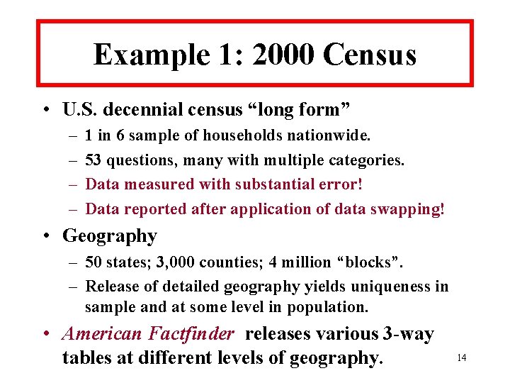
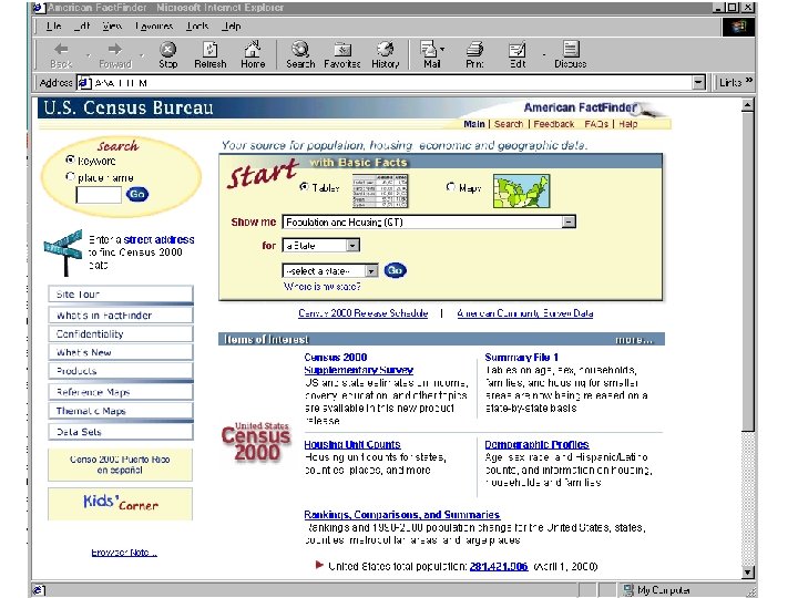
Example 1: 2000 Census • U. S. decennial census “long form” – – 1 in 6 sample of households nationwide. 53 questions, many with multiple categories. Data measured with substantial error! Data reported after application of data swapping! • Geography – 50 states; 3, 000 counties; 4 million “blocks”. – Release of detailed geography yields uniqueness in sample and at some level in population. • American Factfinder releases various 3 -way tables at different levels of geography. 14

15

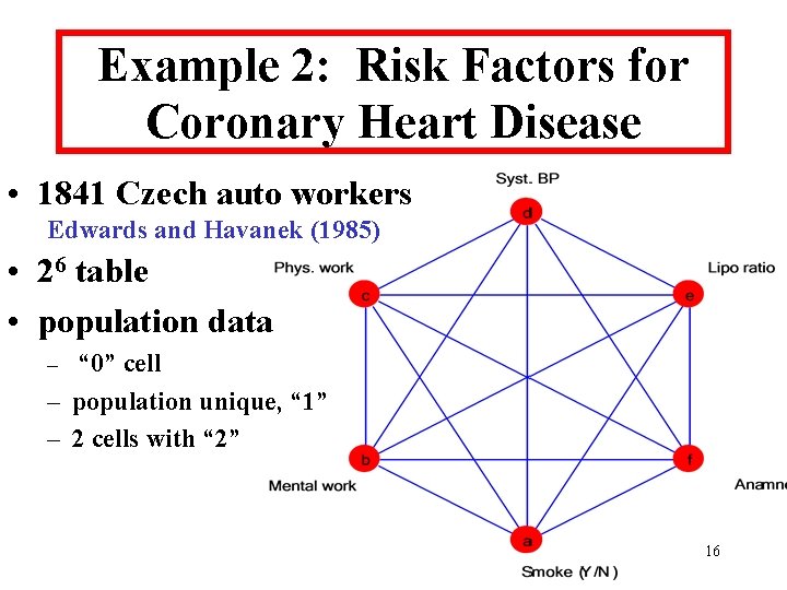
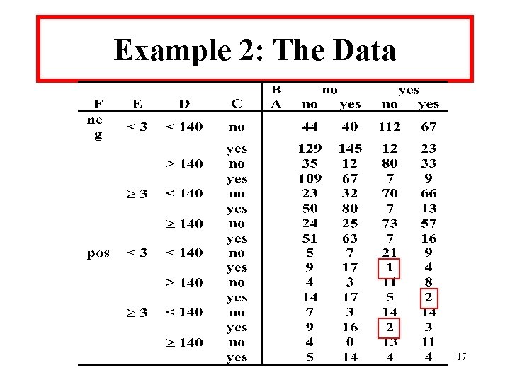
Example 2: Risk Factors for Coronary Heart Disease • 1841 Czech auto workers Edwards and Havanek (1985) • 26 table • population data – “ 0” cell – population unique, “ 1” – 2 cells with “ 2” 16

Example 2: The Data 17

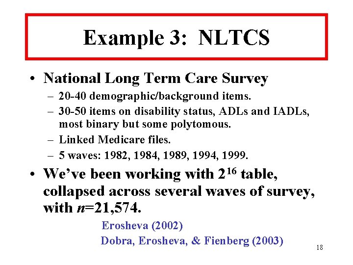
Example 3: NLTCS • National Long Term Care Survey – 20 -40 demographic/background items. – 30 -50 items on disability status, ADLs and IADLs, most binary but some polytomous. – Linked Medicare files. – 5 waves: 1982, 1984, 1989, 1994, 1999. • We’ve been working with 216 table, collapsed across several waves of survey, with n=21, 574. Erosheva (2002) Dobra, Erosheva, & Fienberg (2003) 18

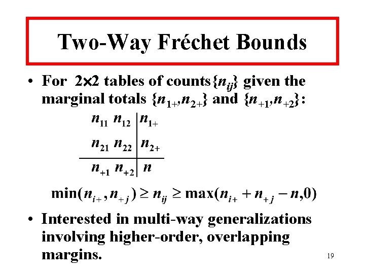
Two-Way Fréchet Bounds • For 2 2 tables of counts{nij} given the marginal totals {n 1+, n 2+} and {n+1, n+2}: • Interested in multi-way generalizations involving higher-order, overlapping margins. 19

Bounds for Multi-Way Tables • k-way table of non-negative counts, k 3. – Release set of marginal totals, possibly overlapping. – Goal: Compute bounds for cell entries. – LP and IP approaches are NP-hard. • Our strategy has been to: – Develop efficient methods for several special cases. – Exploit linkage to statistical theory where possible. – Use general, less efficient methods for residual cases. • Direct generalizations to tables with noninteger, non-negative entries. 20

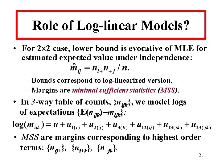
Role of Log-linear Models? • For 2 2 case, lower bound is evocative of MLE for estimated expected value under independence: – Bounds correspond to log-linearized version. – Margins are minimal sufficient statistics (MSS). • In 3 -way table of counts, {nijk}, we model logs of expectations {E(nijk)=mijk}: • MSS are margins corresponding to highest order terms: {nij+}, {ni+k}, {n+jk}. 21

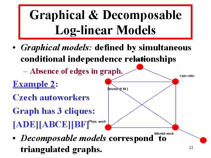
Graphical & Decomposable Log-linear Models • Graphical models: defined by simultaneous conditional independence relationships – Absence of edges in graph. Example 2: Czech autoworkers Graph has 3 cliques: [ADE][ABCE][BF] • Decomposable models correspond to triangulated graphs. 22

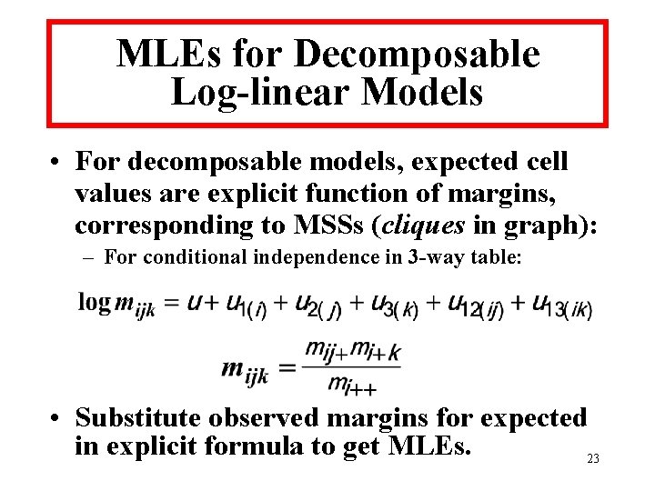
MLEs for Decomposable Log-linear Models • For decomposable models, expected cell values are explicit function of margins, corresponding to MSSs (cliques in graph): – For conditional independence in 3 -way table: • Substitute observed margins for expected in explicit formula to get MLEs. 23

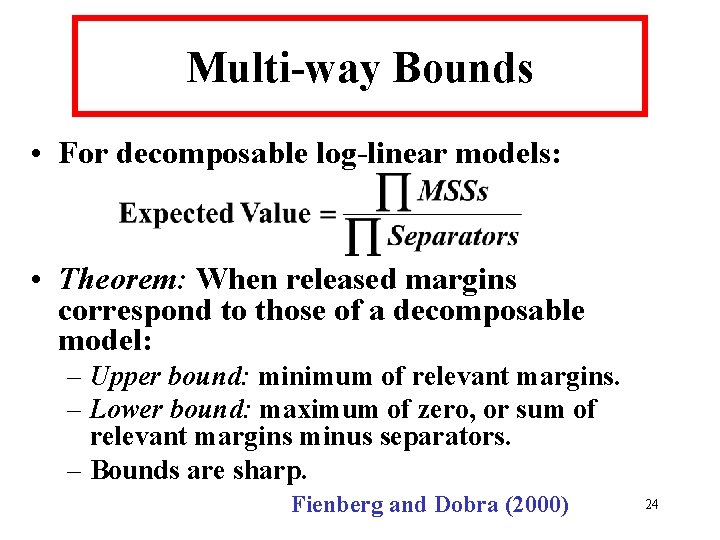
Multi-way Bounds • For decomposable log-linear models: • Theorem: When released margins correspond to those of a decomposable model: – Upper bound: minimum of relevant margins. – Lower bound: maximum of zero, or sum of relevant margins minus separators. – Bounds are sharp. Fienberg and Dobra (2000) 24

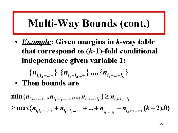
Multi-Way Bounds (cont. ) • Example: Given margins in k-way table that correspond to (k-1)-fold conditional independence given variable 1: • Then bounds are 25

Ex. 2: Czech Autoworkers • Suppose released margins are [ADE][ABCE][BF] : – – Correspond to decomposable graph. Cell containing population unique has bounds [0, 25]. Cells with entry of “ 2” have bounds: [0, 20] and [0, 38]. Lower bounds are all “ 0”. • “Safe” to release these margins; low risk of disclosure. 26

Bounds for [BF][ABCE][ADE] 27

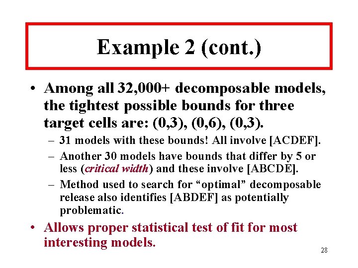
Example 2 (cont. ) • Among all 32, 000+ decomposable models, the tightest possible bounds for three target cells are: (0, 3), (0, 6), (0, 3). – 31 models with these bounds! All involve [ACDEF]. – Another 30 models have bounds that differ by 5 or less (critical width) and these involve [ABCDE]. – Method used to search for “optimal” decomposable release also identifies [ABDEF] as potentially problematic. • Allows proper statistical test of fit for most interesting models. 28

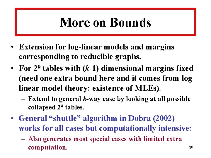
More on Bounds • Extension for log-linear models and margins corresponding to reducible graphs. • For 2 k tables with (k-1) dimensional margins fixed (need one extra bound here and it comes from loglinear model theory: existence of MLEs). – Extend to general k-way case by looking at all possible collapsed 2 k tables. • General “shuttle” algorithm in Dobra (2002) works for all cases but computationally intensive: – Also generates most special cases with limited extra computation. 29

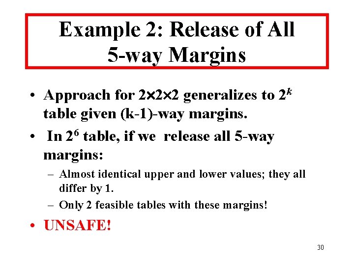
Example 2: Release of All 5 -way Margins • Approach for 2 2 2 generalizes to 2 k table given (k-1)-way margins. • In 26 table, if we release all 5 -way margins: – Almost identical upper and lower values; they all differ by 1. – Only 2 feasible tables with these margins! • UNSAFE! 30

Example 2: Making Proper Statistical Inferences • In Example 2, we know we can’t release [ABCDE] and [ACDEF]. • Suppose we deem release of everything else to be safe, i. e. , we release [ACDE] [ABCDF][ABCEF][BCDEF][ABDEF] and we announce that users can make correct inference from release. • What can user and intruder do? 31

Example 2: Making Proper Statistical Inferences (cont. ) • Includes among models that can be fitted our “favorite”one: [ADE][ABCE][BF]. • Can do proper log-linear inferences using MLE and variation of chi-square tests based on expected values from model linked to released marginals. • Announcement that releases can be used for proper inference will not materially reduce space of possible tables for 32 intruder’s inferences.

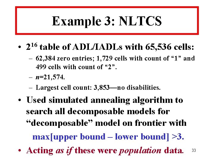
Example 3: NLTCS • 216 table of ADL/IADLs with 65, 536 cells: – 62, 384 zero entries; 1, 729 cells with count of “ 1” and 499 cells with count of “ 2”. – n=21, 574. – Largest cell count: 3, 853—no disabilities. • Used simulated annealing algorithm to search all decomposable models for “decomposable” model on frontier with max[upper bound – lower bound] >3. • Acting as if these were population data. 33

NLTCS Search Results • Decomposable frontier model: {[1, 2, 3, 4, 5, 7, 12], [1, 2, 3, 6, 7, 12], [2, 3, 4, 5, 7, 8], [1, 2, 4, 5, 7, 11], [2, 3, 4, 5, 7, 13], [3, 4, 5, 7, 9, 13], [2, 3, 4, 5, 13, 14], [2, 4, 5, 10, 13, 14], [1, 2, 3, 4, 5, 15], [2, 3, 4, 5, 8, 16]}. • Has one 7 -way and eight 6 -way marginals. 34

Sparseness in NLTCS Data • Sparseness of table in this example extends to margins we might want to release, e. g. , 210 table of ADLs and 26 table of IADLs: – We need to alter margins to allow for release. • Perturbation of table subject to marginal constraints for already-released margins: – Part of framework for NISS prototype. 35

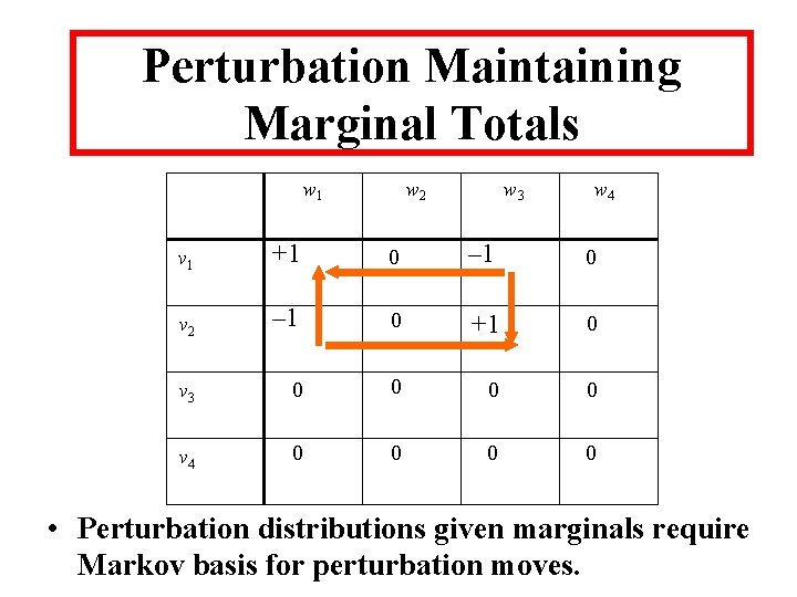
Perturbation Maintaining Marginal Totals w 1 w 2 w 3 w 4 v 1 +1 0 – 1 0 v 2 – 1 0 +1 0 v 3 0 0 v 4 0 0 • Perturbation distributions given marginals require Markov basis for perturbation moves.

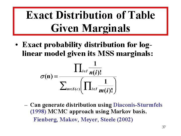
Exact Distribution of Table Given Marginals • Exact probability distribution for loglinear model given its MSS marginals: – Can generate distribution using Diaconis-Sturmfels (1998) MCMC approach using Markov basis. Fienberg, Makov, Meyer, Steele (2002) 37

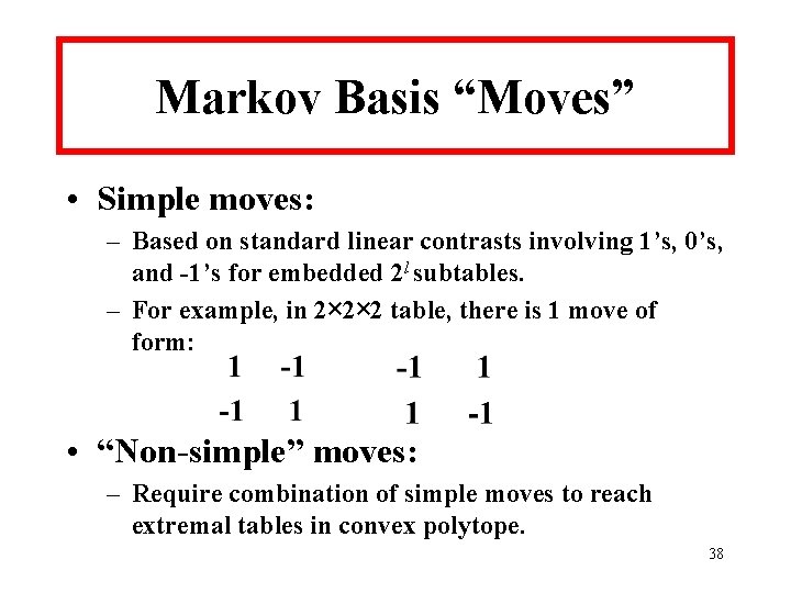
Markov Basis “Moves” • Simple moves: – Based on standard linear contrasts involving 1’s, 0’s, and -1’s for embedded 2 l subtables. – For example, in 2× 2× 2 table, there is 1 move of form: • “Non-simple” moves: – Require combination of simple moves to reach extremal tables in convex polytope. 38

Perturbation for Protection • Perturbation preserving marginals involves a parallel set of results to those for bounds: – Markov basis elements for decomposable case requires only “simple” moves. (Dobra, 2002) – Efficient generation of Markov basis for reducible case. (Dobra and Sullivent, 2002) – Simplifications for 2 k tables (“binomials”). – Rooted in ideas from likelihood theory for log-linear models and computational algebra of toric ideals. 39

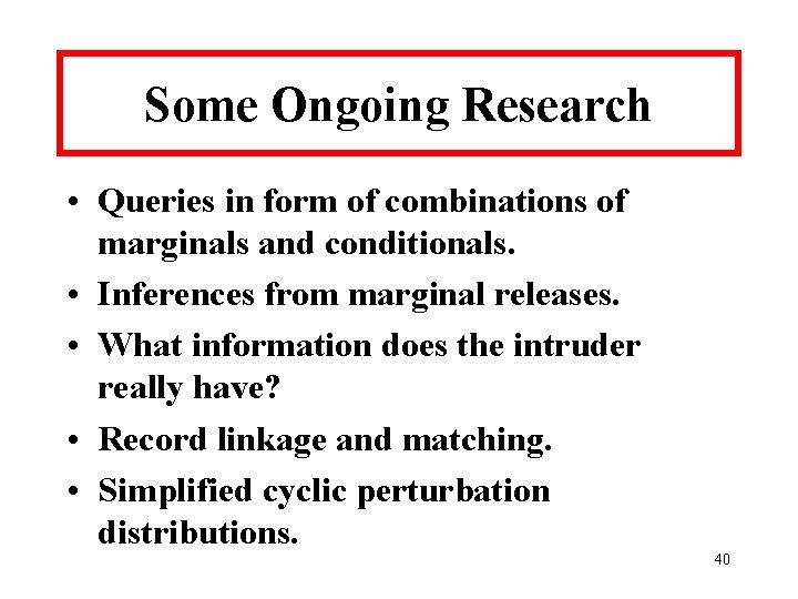
Some Ongoing Research • Queries in form of combinations of marginals and conditionals. • Inferences from marginal releases. • What information does the intruder really have? • Record linkage and matching. • Simplified cyclic perturbation distributions. 40

Some General Principles for Developing DL Methods • All data are informative for intruder including, non-release or suppression. • Need to define and understand potential statistical uses of data in advance: – Leads to useful reportable summaries. • Methods should allow for reversibility for inference purposes: – Missing data should be “ignorable” for inferences. – Assessing goodness of fit is important. 41

Where Will Tools Come From? • Statistical methods and theory and modern datamining methods. • Optimization approaches from OR. • New mathematics, e. g. , computational algebraic geometry. 42

Summary • Presented some fundamental abstractions for disclosure limitation. • Illustrated what I refer to as statistical approach to DL using tables of counts. – New theoretical links among disclosure limitation, statistical theory, and computational algebraic geometry. • Articulates some general principles for developing DL methods. 43

The End • Most papers available for downloading at http: //www. niss. org http: //www. stat. cmu. edu/~fienberg/disclosure. html Workshop on Computational Algebraic Statistics December 14 to 18, 2003 American Institute of Mathematics Palo Alto, California http: //aimath. org/ARCC/workshops/compalgstat. html 44

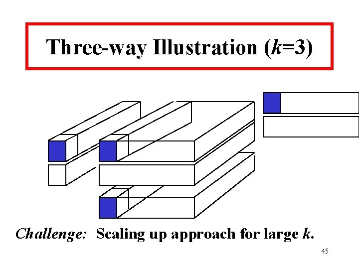
Three-way Illustration (k=3) Challenge: Scaling up approach for large k. 45

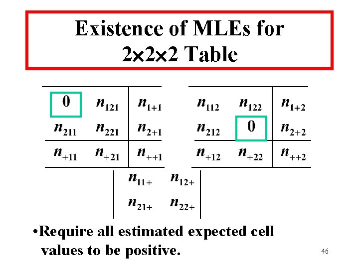
Existence of MLEs for 2 2 2 Table • Require all estimated expected cell values to be positive. 46

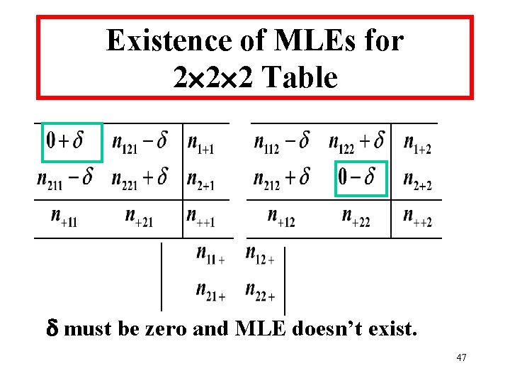
Existence of MLEs for 2 2 2 Table must be zero and MLE doesn’t exist. 47

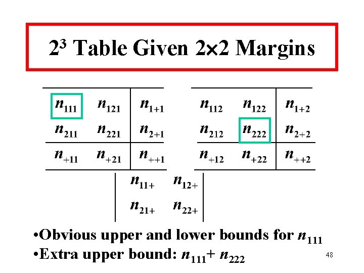
3 2 Table Given 2 2 Margins • Obvious upper and lower bounds for n 111 48 • Extra upper bound: n 111+ n 222

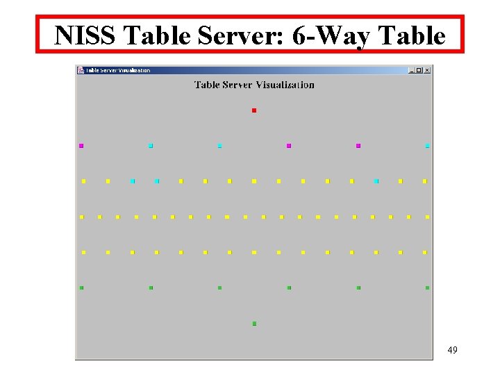
NISS Table Server: 6 -Way Table 49