Statistical Data Analysis Prof Dr Nizamettin AYDIN naydinyildiz

Statistical Data Analysis Prof. Dr. Nizamettin AYDIN naydin@yildiz. edu. tr http: //www 3. yildiz. edu. tr/~naydin 1

Analysis of Variance (ANOVA) 2

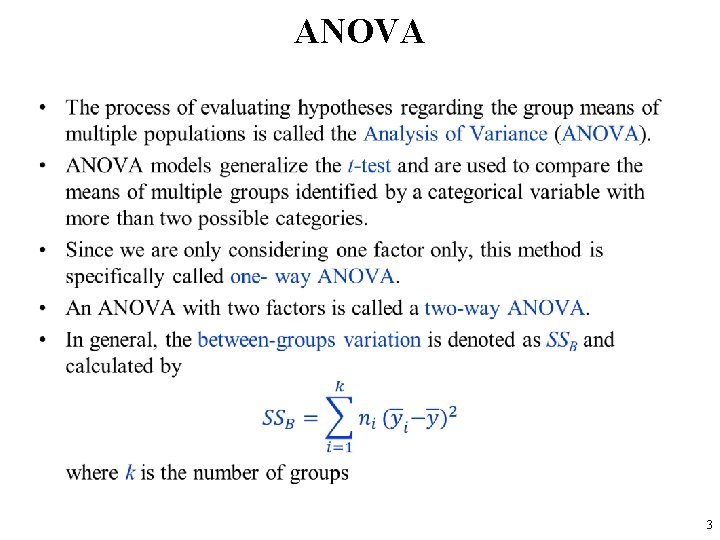
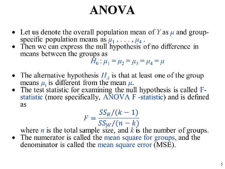
ANOVA • 3

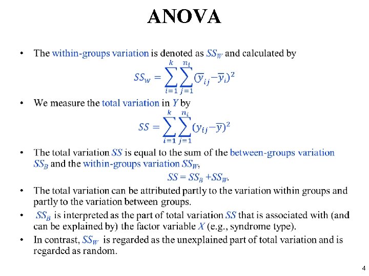
ANOVA • 4

ANOVA • 5

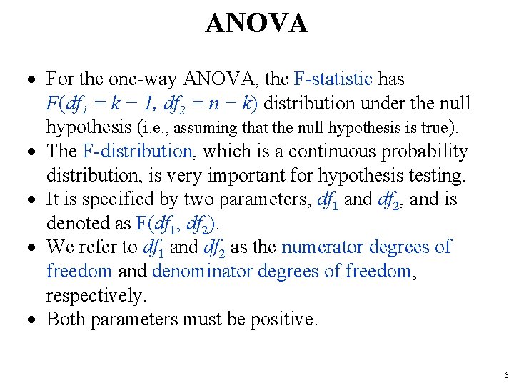
ANOVA For the one-way ANOVA, the F-statistic has F(df 1 = k − 1, df 2 = n − k) distribution under the null hypothesis (i. e. , assuming that the null hypothesis is true). The F-distribution, which is a continuous probability distribution, is very important for hypothesis testing. It is specified by two parameters, df 1 and df 2, and is denoted as F(df 1, df 2). We refer to df 1 and df 2 as the numerator degrees of freedom and denominator degrees of freedom, respectively. Both parameters must be positive. 6

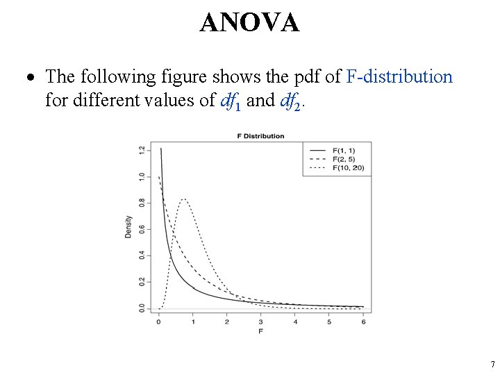
ANOVA The following figure shows the pdf of F-distribution for different values of df 1 and df 2. 7

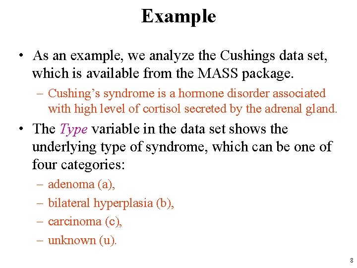
Example • As an example, we analyze the Cushings data set, which is available from the MASS package. – Cushing’s syndrome is a hormone disorder associated with high level of cortisol secreted by the adrenal gland. • The Type variable in the data set shows the underlying type of syndrome, which can be one of four categories: – – adenoma (a), bilateral hyperplasia (b), carcinoma (c), unknown (u). 8

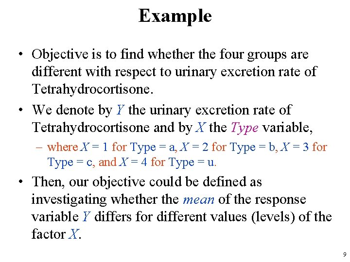
Example • Objective is to find whether the four groups are different with respect to urinary excretion rate of Tetrahydrocortisone. • We denote by Y the urinary excretion rate of Tetrahydrocortisone and by X the Type variable, – where X = 1 for Type = a, X = 2 for Type = b, X = 3 for Type = c, and X = 4 for Type = u. • Then, our objective could be defined as investigating whether the mean of the response variable Y differs for different values (levels) of the factor X. 9

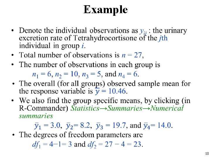
Example • 10

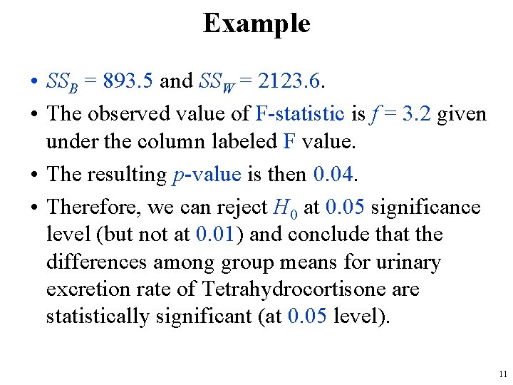
Example • SSB = 893. 5 and SSW = 2123. 6. • The observed value of F-statistic is f = 3. 2 given under the column labeled F value. • The resulting p-value is then 0. 04. • Therefore, we can reject H 0 at 0. 05 significance level (but not at 0. 01) and conclude that the differences among group means for urinary excretion rate of Tetrahydrocortisone are statistically significant (at 0. 05 level). 11

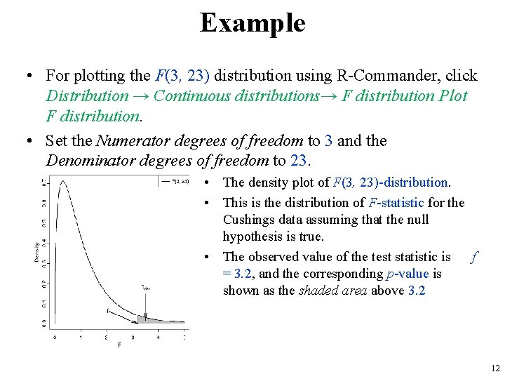
Example • For plotting the F(3, 23) distribution using R-Commander, click Distribution → Continuous distributions→ F distribution Plot F distribution. • Set the Numerator degrees of freedom to 3 and the Denominator degrees of freedom to 23. • The density plot of F(3, 23)-distribution. • This is the distribution of F-statistic for the Cushings data assuming that the null hypothesis is true. • The observed value of the test statistic is f = 3. 2, and the corresponding p-value is shown as the shaded area above 3. 2 12