Statistical Data Analysis Prof Dr Nizamettin AYDIN naydinyildiz

Statistical Data Analysis Prof. Dr. Nizamettin AYDIN naydin@yildiz. edu. tr http: //www 3. yildiz. edu. tr/~naydin 1

Regression Analysis 2

Regression Analysis • The modeling of the relationship between a response variable and a set of explanatory variables is one of the most widely used of all statistical techniques. – We refer to this type of modeling as regression analysis. • A regression model provides the user with a functional relationship between the response variable and explanatory variables that allows the user to determine which of the explanatory variables have an effect on the response. – The regression model allows the user to explore what happens to the response variable for specified changes in the explanatory variables. • {For example, financial officers must predict future cash flows based on specified values of interest rates, raw material costs, salary increases, and so on} 3

Regression Analysis • The basic idea of regression analysis is to obtain a model for the functional relationship between a response variable (often referred to as the dependent variable) and one or more explanatory variables (often referred to as the independent variables). • Regression models have a number of uses: – The model provides a description of the major features of the data set. • In some cases, a subset of the explanatory variables will not affect the response variable, and, hence, the researcher will not have to measure or control any of these variables in future studies. – This may result in significant savings in future studies or experiments. 4

Regression Analysis – The equation relating the response variable to the explanatory variables produced from the regression analysis provides estimates of the response variable for values of the explanatory variables not observed in the study. • For example, a clinical trial is designed to study the response of a subject to various dose levels of a new drug. • Because of time and budgetary constraints, only a limited number of dose levels are used in the study. – The regression equation will provide estimates of the subjects’ response for dose levels not included in the study. – In business applications, the prediction of future sales of a product is crucial to production planning. • If the data provide a model that has a good fit in relating current sales to sales in previous months, prediction of sales in future months is possible. 5

Regression Analysis – In some applications of regression analysis, the researcher is seeking a model that can accurately estimate the values of a variable that is difficult or expensive to measure using explanatory variables that are inexpensive to measure and obtain. • If such a model is obtained, then in future applications it is possible to avoid having to obtain the values of the expensive variable by measuring the values of the inexpensive variables and using the regression equation to estimate the values of the expensive variable. – For example, a physical fitness center wants to determine the physical wellbeing of its new clients. – Maximal oxygen uptake is recognized as the single best measure of cardiorespiratory fitness, but its measurement is expensive. – Therefore, the director of the fitness center would want a model that provides accurate estimates of maximal oxygen uptake using easily measured variables such as weight, age, heart rate after a 1 -mile walk, time needed to walk 1 mile, and so on. 6

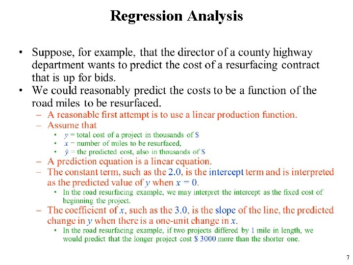
Regression Analysis • 7

Regression Analysis • After this soft introduction, we now discuss linear regression models for either testing a hypothesis regarding the relationship between one or more explanatory variables and a response variable, or predicting unknown values of the response variable using one or more predictors. – We use X to denote explanatory variables and Y to denote response variables. • We start by focusing on problems where the explanatory variable is binary. – As before, the binary variable X can be either 0 or 1. • We then continue our discussion for situations where the explanatory variable is numerical. 8

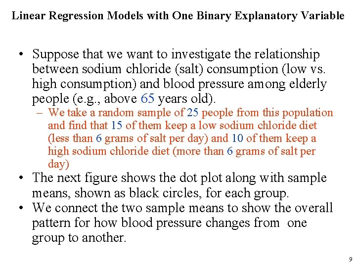
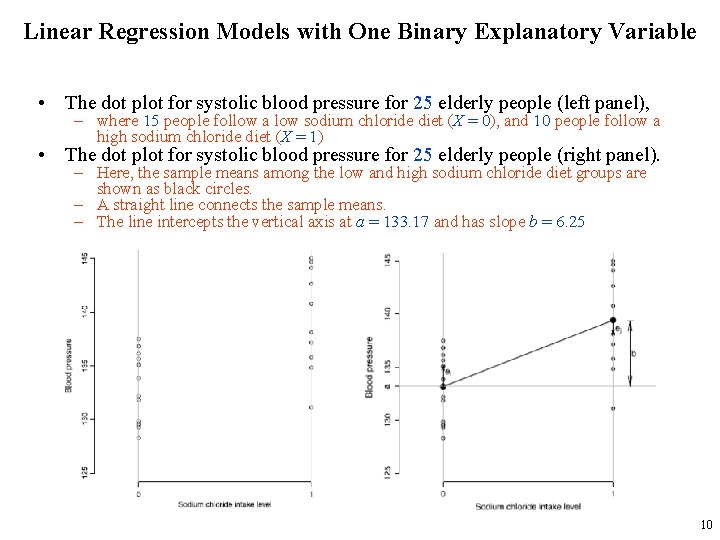
Linear Regression Models with One Binary Explanatory Variable • Suppose that we want to investigate the relationship between sodium chloride (salt) consumption (low vs. high consumption) and blood pressure among elderly people (e. g. , above 65 years old). – We take a random sample of 25 people from this population and find that 15 of them keep a low sodium chloride diet (less than 6 grams of salt per day) and 10 of them keep a high sodium chloride diet (more than 6 grams of salt per day) • The next figure shows the dot plot along with sample means, shown as black circles, for each group. • We connect the two sample means to show the overall pattern for how blood pressure changes from one group to another. 9

Linear Regression Models with One Binary Explanatory Variable • The dot plot for systolic blood pressure for 25 elderly people (left panel), – where 15 people follow a low sodium chloride diet (X = 0), and 10 people follow a high sodium chloride diet (X = 1) • The dot plot for systolic blood pressure for 25 elderly people (right panel). – Here, the sample means among the low and high sodium chloride diet groups are shown as black circles. – A straight line connects the sample means. – The line intercepts the vertical axis at a = 133. 17 and has slope b = 6. 25 10

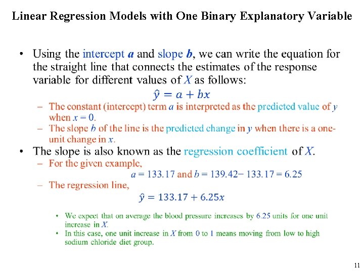
Linear Regression Models with One Binary Explanatory Variable • 11

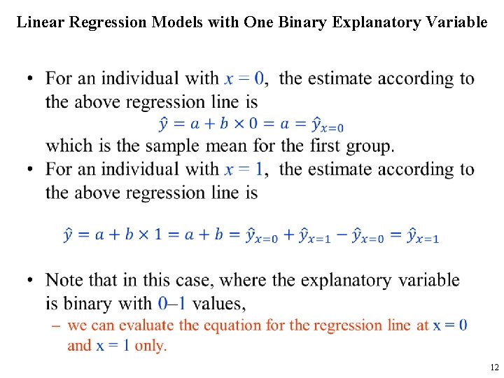
Linear Regression Models with One Binary Explanatory Variable • 12

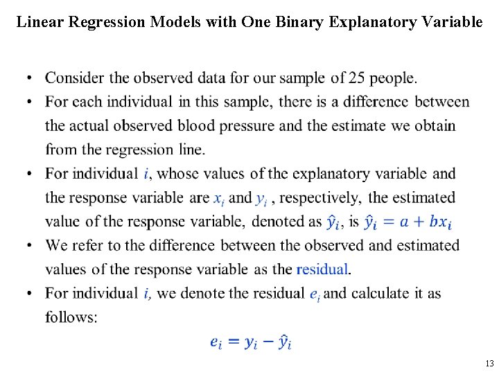
Linear Regression Models with One Binary Explanatory Variable • 13

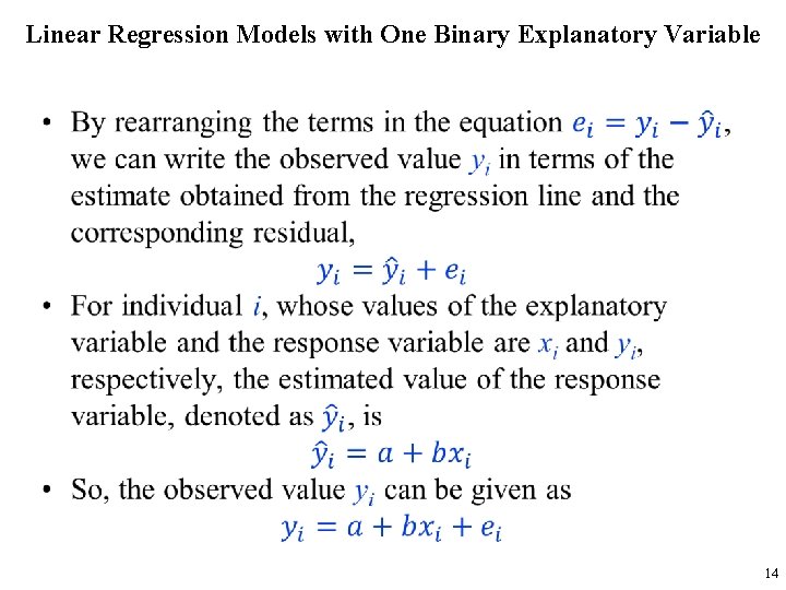
Linear Regression Models with One Binary Explanatory Variable • 14

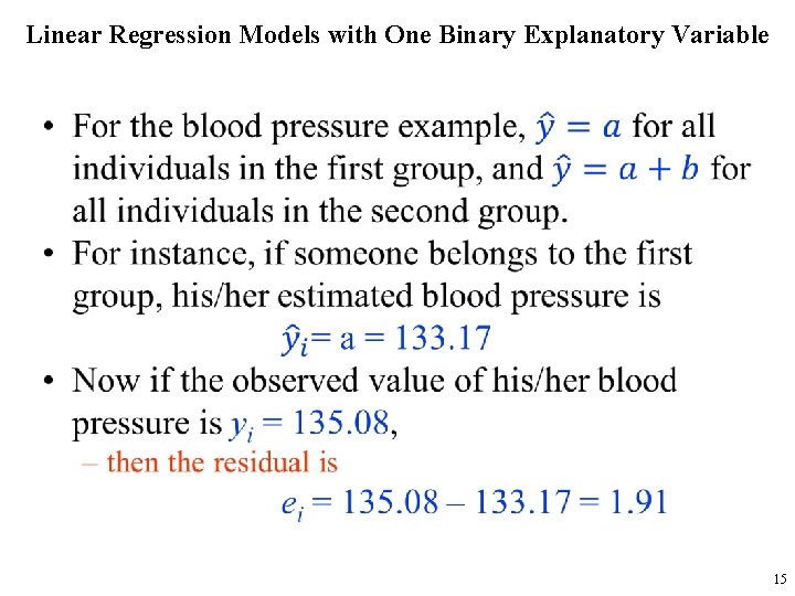
Linear Regression Models with One Binary Explanatory Variable • 15

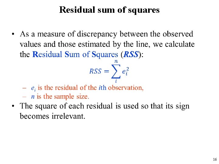
Residual sum of squares • 16

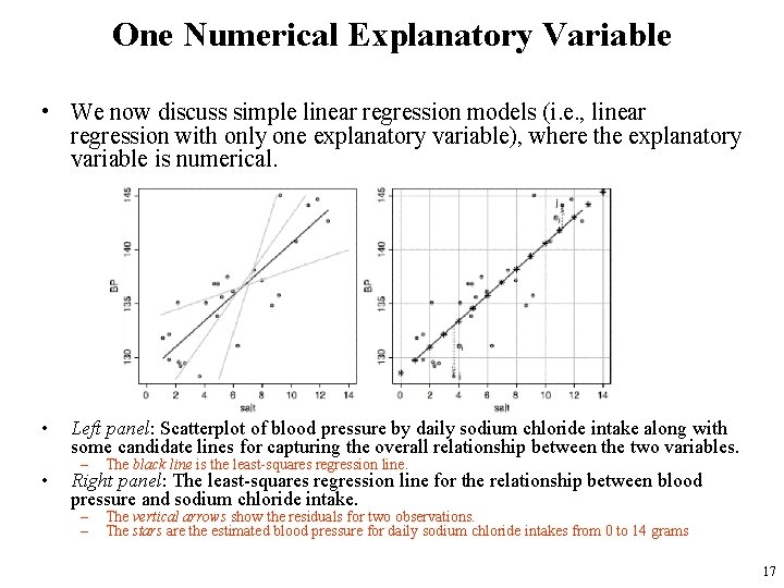
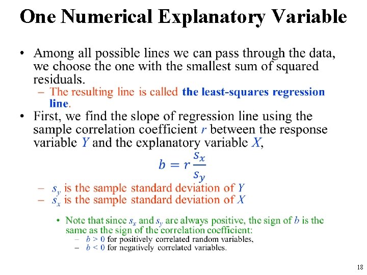
One Numerical Explanatory Variable • We now discuss simple linear regression models (i. e. , linear regression with only one explanatory variable), where the explanatory variable is numerical. • • Left panel: Scatterplot of blood pressure by daily sodium chloride intake along with some candidate lines for capturing the overall relationship between the two variables. – The black line is the least-squares regression line. – – The vertical arrows show the residuals for two observations. The stars are the estimated blood pressure for daily sodium chloride intakes from 0 to 14 grams Right panel: The least-squares regression line for the relationship between blood pressure and sodium chloride intake. 17

One Numerical Explanatory Variable • 18

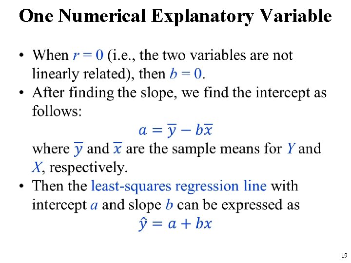
One Numerical Explanatory Variable • 19

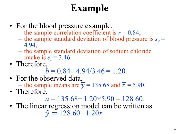
Example • 20

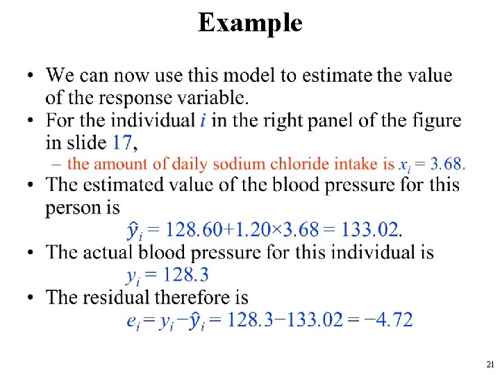
Example • 21

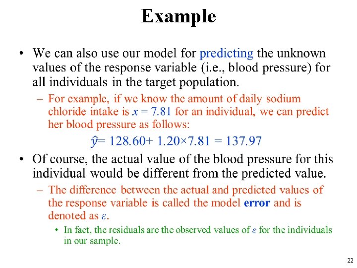
Example • 22

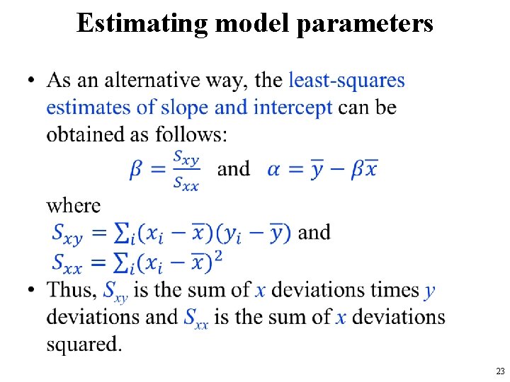
Estimating model parameters • 23

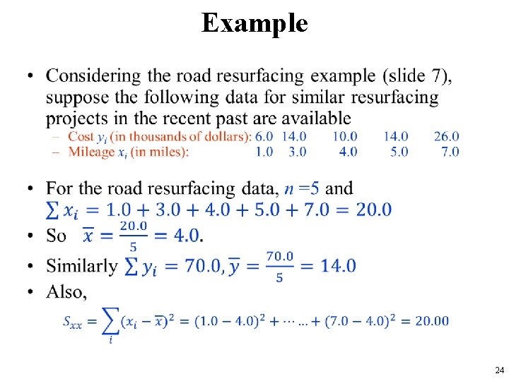
Example • 24

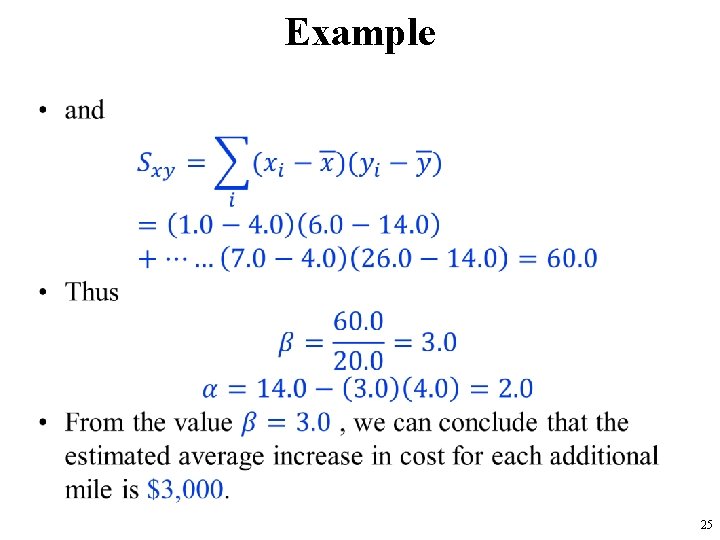
Example • 25

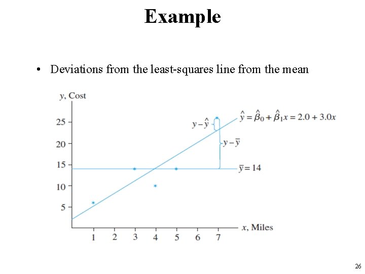
Example • Deviations from the least-squares line from the mean 26

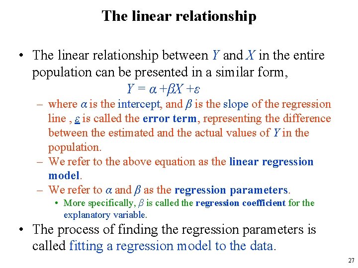
The linear relationship • The linear relationship between Y and X in the entire population can be presented in a similar form, Y = α +βX +ε – where α is the intercept, and β is the slope of the regression line , ε is called the error term, representing the difference between the estimated and the actual values of Y in the population. – We refer to the above equation as the linear regression model. – We refer to α and β as the regression parameters. • More specifically, β is called the regression coefficient for the explanatory variable. • The process of finding the regression parameters is called fitting a regression model to the data. 27

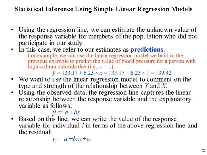
Statistical Inference Using Simple Linear Regression Models • 28

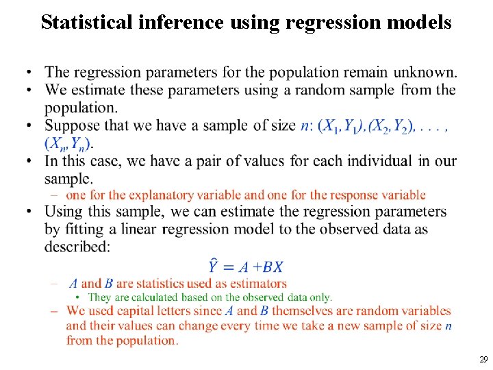
Statistical inference using regression models • 29

Statistical inference using regression models • The point estimates do not reflect our uncertainty; – we always remain uncertain about the actual values of α and β, and our estimates for these parameters can change when we take a different sample from the population. • Therefore, we use the point estimates a and b obtained from the observed data along with the sampling distribution of the estimators A and B to find confidence interval estimates for α and β. – This is similar to what we had for the population mean. • Because the slope parameter β has a central role in capturing the linear relationship between Y and X, we need to find its confidence intervals. – Similar approach can be used for the intercept α. 30

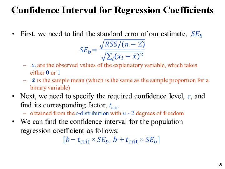
Confidence Interval for Regression Coefficients • 31

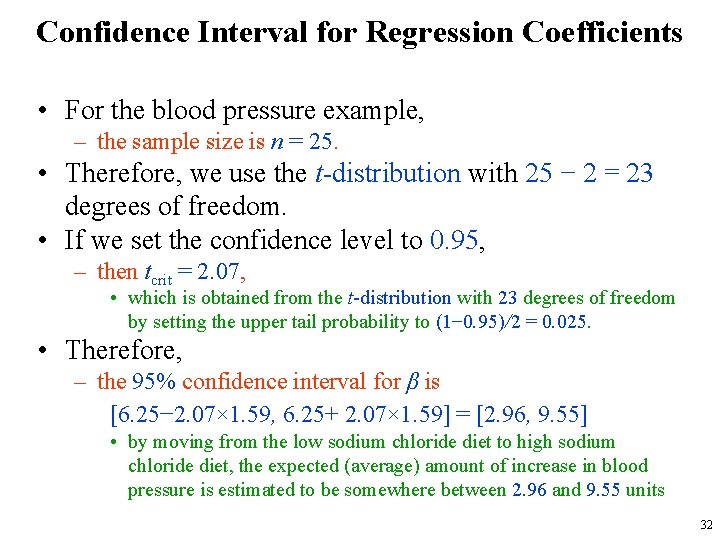
Confidence Interval for Regression Coefficients • For the blood pressure example, – the sample size is n = 25. • Therefore, we use the t-distribution with 25 − 2 = 23 degrees of freedom. • If we set the confidence level to 0. 95, – then tcrit = 2. 07, • which is obtained from the t-distribution with 23 degrees of freedom by setting the upper tail probability to (1− 0. 95)/2 = 0. 025. • Therefore, – the 95% confidence interval for β is [6. 25− 2. 07× 1. 59, 6. 25+ 2. 07× 1. 59] = [2. 96, 9. 55] • by moving from the low sodium chloride diet to high sodium chloride diet, the expected (average) amount of increase in blood pressure is estimated to be somewhere between 2. 96 and 9. 55 units 32

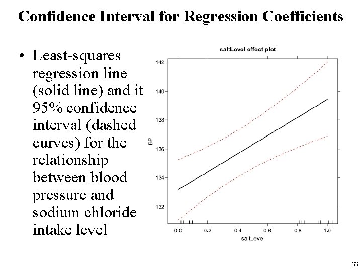
Confidence Interval for Regression Coefficients • Least-squares regression line (solid line) and its 95% confidence interval (dashed curves) for the relationship between blood pressure and sodium chloride intake level 33

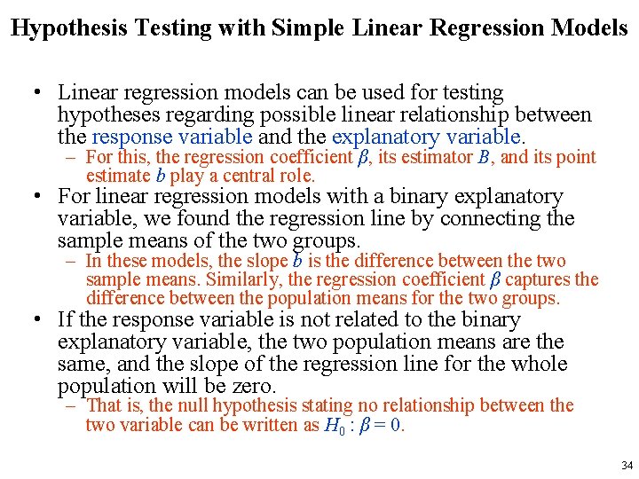
Hypothesis Testing with Simple Linear Regression Models • Linear regression models can be used for testing hypotheses regarding possible linear relationship between the response variable and the explanatory variable. – For this, the regression coefficient β, its estimator B, and its point estimate b play a central role. • For linear regression models with a binary explanatory variable, we found the regression line by connecting the sample means of the two groups. – In these models, the slope b is the difference between the two sample means. Similarly, the regression coefficient β captures the difference between the population means for the two groups. • If the response variable is not related to the binary explanatory variable, the two population means are the same, and the slope of the regression line for the whole population will be zero. – That is, the null hypothesis stating no relationship between the two variable can be written as H 0 : β = 0. 34

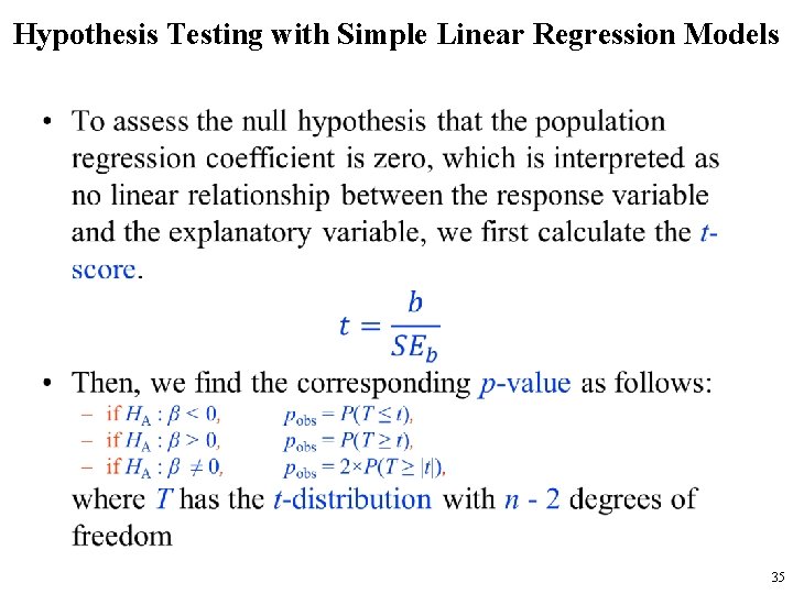
Hypothesis Testing with Simple Linear Regression Models • 35

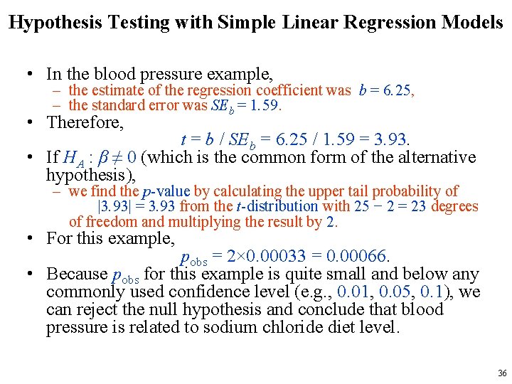
Hypothesis Testing with Simple Linear Regression Models • In the blood pressure example, – the estimate of the regression coefficient was b = 6. 25, – the standard error was SEb = 1. 59. • Therefore, t = b / SEb = 6. 25 / 1. 59 = 3. 93. • If HA : β ≠ 0 (which is the common form of the alternative hypothesis), – we find the p-value by calculating the upper tail probability of |3. 93| = 3. 93 from the t-distribution with 25 − 2 = 23 degrees of freedom and multiplying the result by 2. • For this example, pobs = 2× 0. 00033 = 0. 00066. • Because pobs for this example is quite small and below any commonly used confidence level (e. g. , 0. 01, 0. 05, 0. 1), we can reject the null hypothesis and conclude that blood pressure is related to sodium chloride diet level. 36

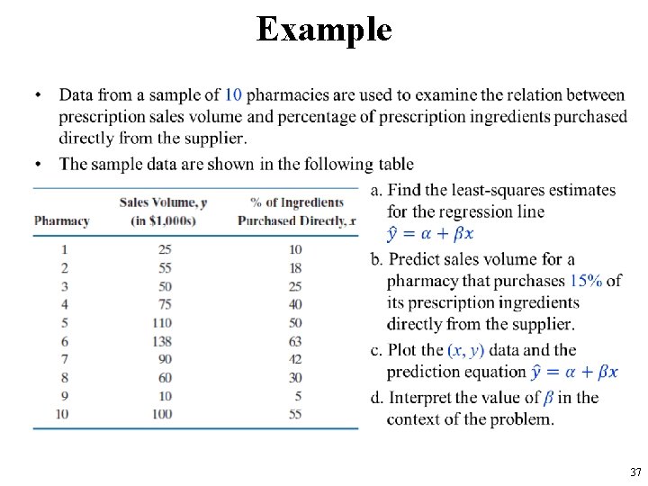
Example • 37

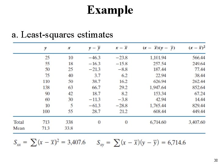
Example a. Least-squares estimates 38

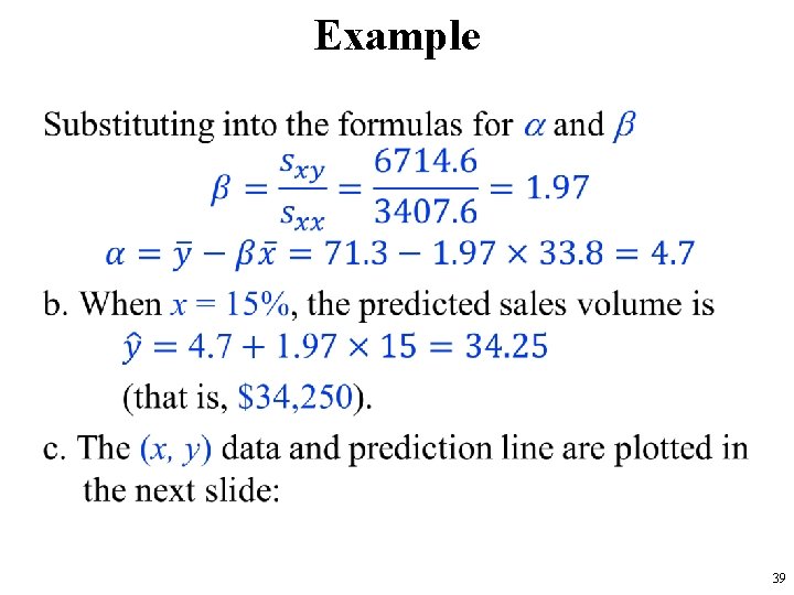
Example • 39

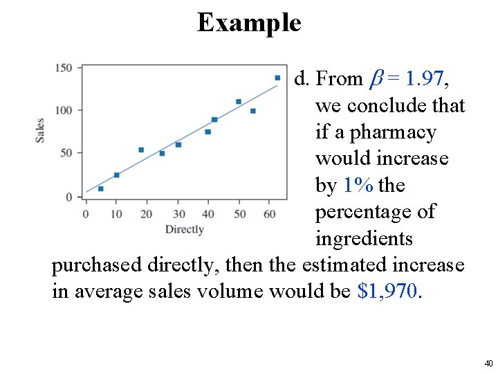
Example d. From b = 1. 97, we conclude that if a pharmacy would increase by 1% the percentage of ingredients purchased directly, then the estimated increase in average sales volume would be $1, 970. 40

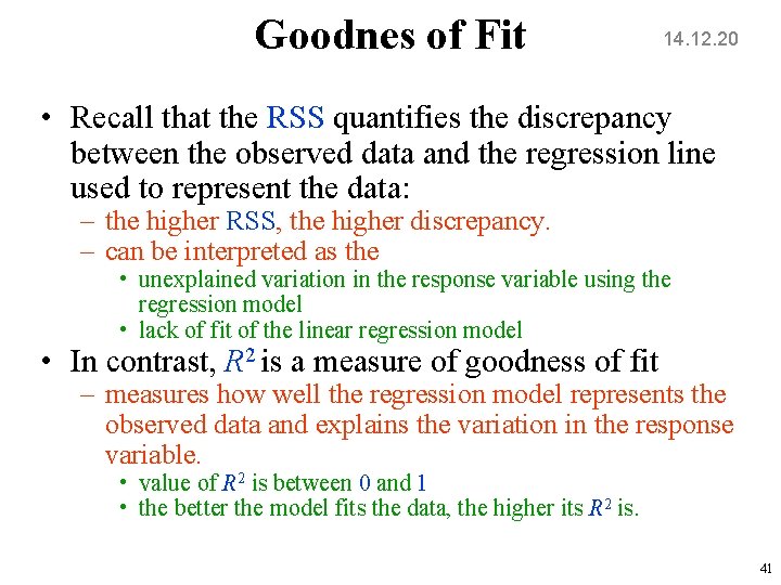
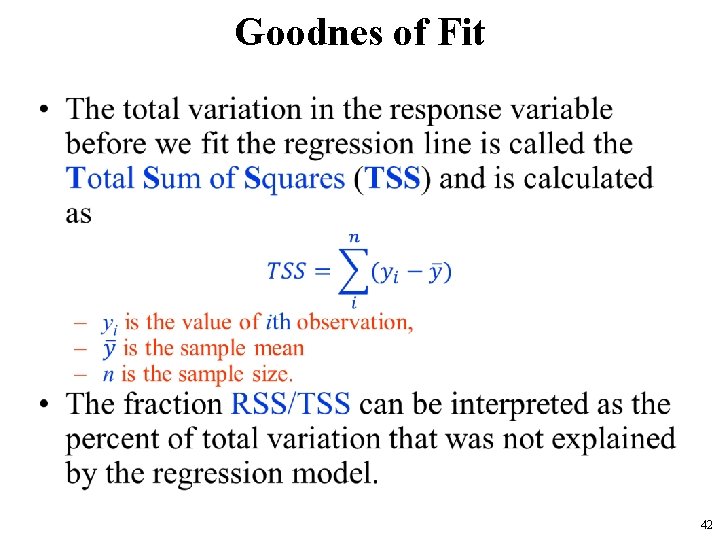
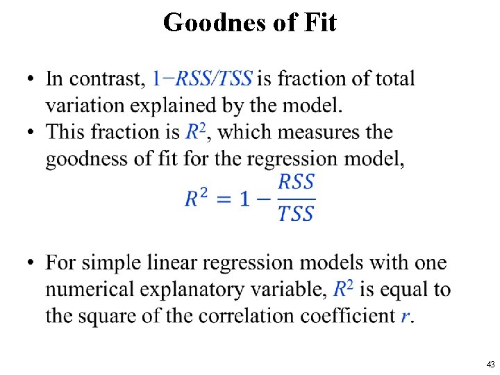
Goodnes of Fit 14. 12. 20 • Recall that the RSS quantifies the discrepancy between the observed data and the regression line used to represent the data: – the higher RSS, the higher discrepancy. – can be interpreted as the • unexplained variation in the response variable using the regression model • lack of fit of the linear regression model • In contrast, R 2 is a measure of goodness of fit – measures how well the regression model represents the observed data and explains the variation in the response variable. • value of R 2 is between 0 and 1 • the better the model fits the data, the higher its R 2 is. 41

Goodnes of Fit • 42

Goodnes of Fit • 43

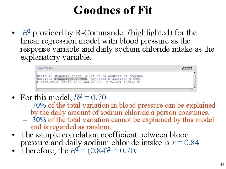
Goodnes of Fit • R 2 provided by R-Commander (highlighted) for the linear regression model with blood pressure as the response variable and daily sodium chloride intake as the explanatory variable. • For this model, R 2 = 0. 70. – 70% of the total variation in blood pressure can be explained by the daily amount of sodium chloride a person consumes. – 30% of the total variation cannot be explained by this model and is regarded as random. • The sample correlation coefficient between blood pressure and daily sodium chloride intake is r = 0. 84. • Therefore, the R 2 = (0. 84)2 = 0. 70. 44

Model Assumptions and Diagnostics • Statistical inference using linear regression models is based on several assumptions: – Linearity – Independence – Constant Variance and Normality • Violating these assumptions could lead to wrong conclusions. 45

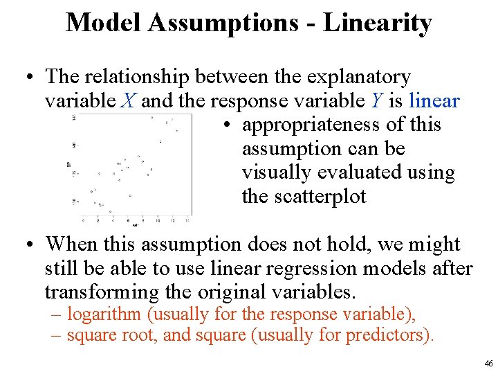
Model Assumptions - Linearity • The relationship between the explanatory variable X and the response variable Y is linear • appropriateness of this assumption can be visually evaluated using the scatterplot • When this assumption does not hold, we might still be able to use linear regression models after transforming the original variables. – logarithm (usually for the response variable), – square root, and square (usually for predictors). 46

Model Assumptions - Independence • a reasonable assumption if – simple random sampling is used to select individuals that are not related to each other – multiple observations are not obtained from the same individual. • However, we sometimes sample – related subjects in groups – unrelated subjects, but obtain multiple measurements of the response variable for each subject. • For such data, regression models taking the dependencies among observations into account should be used. – When multiple observations are obtained over time, a class of statistical models called longitudinal models is used. 47

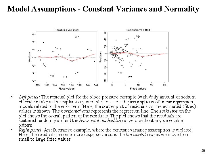
Model Assumptions - Constant Variance and Normality • Using linear regression models also involves some assumptions regarding the probability distribution of the response variable Y, which is the main random variable in regression analysis. • It is expected that the variation of the actual values of the response variable around the regression line remains the same regardless of the value of the explanatory variable. – This is called the constant variance assumption, which is also known as the homoscedasticity assumption. • Heteroscedasticity refers to situations where the constant variance assumption is violated. • To check the validity of these assumptions, the residuals e that are observed values of the random variable ε is examined. 48

Model Assumptions - Constant Variance and Normality • To illustrate how we check the assumptions regarding ε, we use the blood pressure example with daily amount of sodium chloride intake as the explanatory variable. • In R-Commander, make sure Reg. Model. 2 is the active model, then click Models→Graphs Basic diagnostic plots • This creates several model diagnostic plots shown in the next slide. • When the constant variance assumption does not hold, we can sometimes stabilize the variance using simple transformations of the response variable so the variance becomes approximately constant. – For example, instead of Y , we could use sqrt(Y) or log(Y) in the regression model. 49

Model Assumptions - Constant Variance and Normality • • Left panel: The residual plot for the blood pressure example (with daily amount of sodium chloride intake as the explanatory variable) to assess the assumptions of linear regression models related to the error term. Here, the scatter plot of residuals vs. the estimated (fitted) values is shown. The horizontal axis represents the regression line. The solid line on the plot shows the overall pattern of the residuals. The plot shows that the residuals are scattered randomly around the horizontal dashed line at zero without any detectable pattern. Right panel: An illustrative example, where the constant variance assumption is violated. Here, the residuals become more dispersed around the horizontal line as we move from small to large fitted values 50

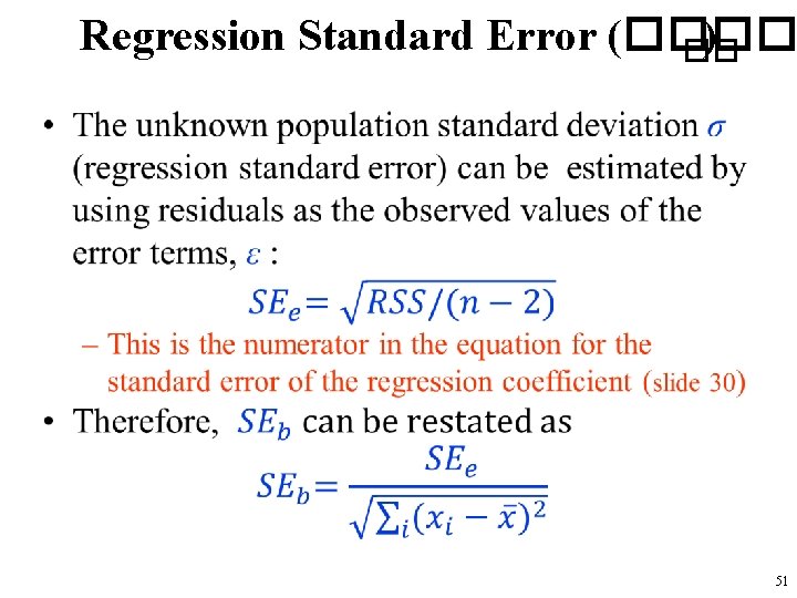
Regression Standard Error (���� ) �� • 51

Multiple Linear Regression • In most cases, we are interested in the relationship between the response variable and multiple explanatory variables. • If our objective is to predict unknown values of the response variable, we might be able to improve prediction accuracy by including multiple predictors in the linear regression model. • Models with multiple explanatory variables or predictors are called multiple linear regression models. 52

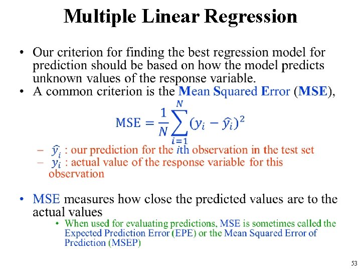
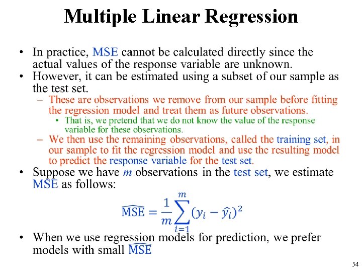
Multiple Linear Regression • 53

Multiple Linear Regression • 54

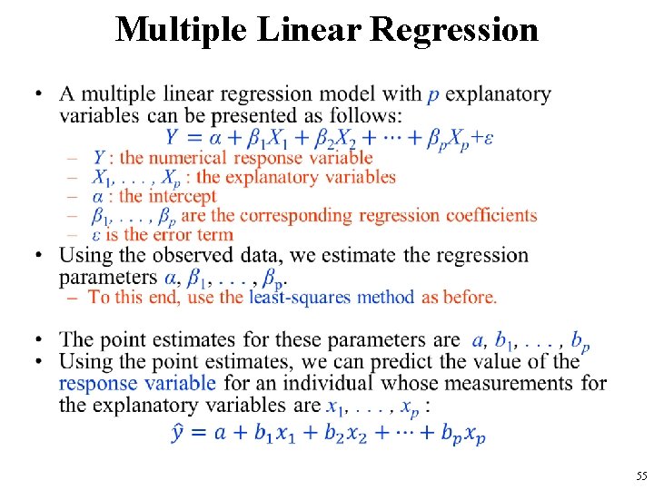
Multiple Linear Regression • 55

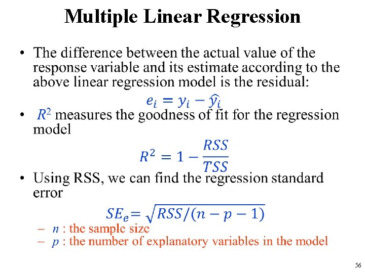
Multiple Linear Regression • 56

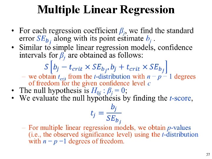
Multiple Linear Regression • 57

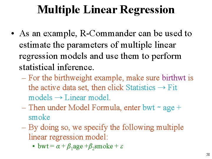
Multiple Linear Regression • As an example, R-Commander can be used to estimate the parameters of multiple linear regression models and use them to perform statistical inference. – For the birthweight example, make sure birthwt is the active data set, then click Statistics → Fit models → Linear model. – Then under Model Formula, enter bwt ∼ age + smoke – By doing so, we specify the following multiple linear regression model: • bwt = α + β 1 age +β 2 smoke + ε 58

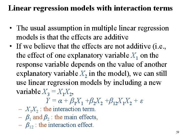
Linear regression models with interaction terms • The usual assumption in multiple linear regression models is that the effects are additive • If we believe that the effects are not additive (i. e. , the effect of one explanatory variable X 1 on the response variable depends on the value of another explanatory variable X 2 in the model), we can still use linear regression models by including a new variable X 3 = X 1 X 2, Y = α + β 1 X 1 +β 2 X 2 +β 12 X 1 X 2 + ε – X 1 X 2 : the interaction term. – β 1 and β 2 : the main effects, – β 12 : the interaction effect. 59

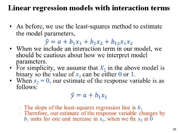
Linear regression models with interaction terms • 60

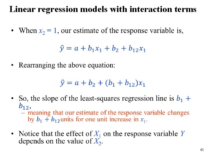
Linear regression models with interaction terms • 61

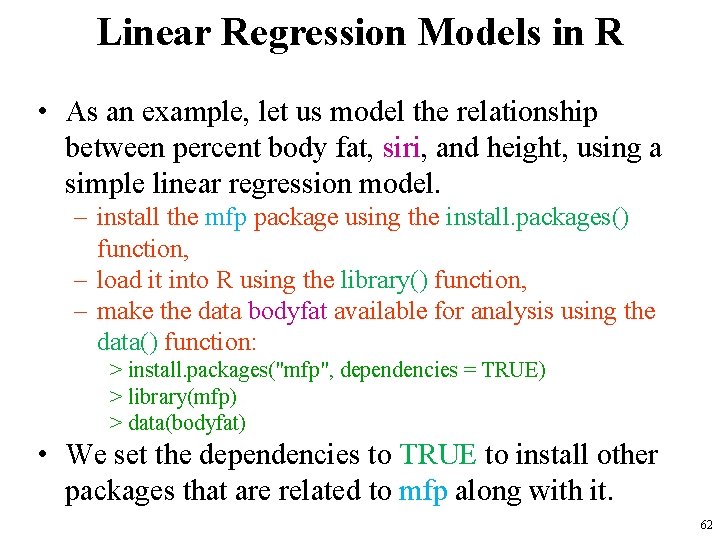
Linear Regression Models in R • As an example, let us model the relationship between percent body fat, siri, and height, using a simple linear regression model. – install the mfp package using the install. packages() function, – load it into R using the library() function, – make the data bodyfat available for analysis using the data() function: > install. packages("mfp", dependencies = TRUE) > library(mfp) > data(bodyfat) • We set the dependencies to TRUE to install other packages that are related to mfp along with it. 62

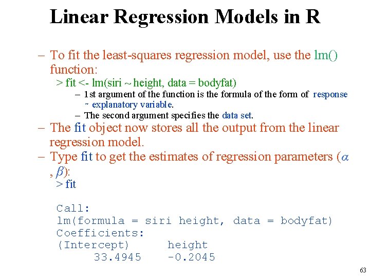
Linear Regression Models in R – To fit the least-squares regression model, use the lm() function: > fit <- lm(siri ~ height, data = bodyfat) – 1 st argument of the function is the formula of the form of response ∼ explanatory variable. – The second argument specifies the data set. – The fit object now stores all the output from the linear regression model. – Type fit to get the estimates of regression parameters (α , β): > fit Call: lm(formula = siri height, data = bodyfat) Coefficients: (Intercept) height 33. 4945 -0. 2045 63

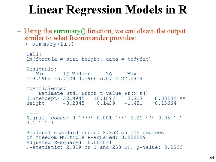
Linear Regression Models in R – Using the summary() function, we can obtain the output similar to what Rcommander provides: > summary(fit) Call: lm(formula = siri height, data = bodyfat) Residuals: Min 1 Q Median 3 Q Max -19. 5902 -6. 7124 0. 3966 6. 0716 27. 0919 Coefficients: Estimate Std. Error t value Pr(>|t|) (Intercept) 33. 4945 10. 1096 3. 313 height -0. 2045 0. 1439 -1. 421 0. 00106 ** 0. 15664 –--Signif. codes: 0 ’***’ 0. 001 ’**’ 0. 01 ’*’ 0. 05 ’. ’ 0. 1 ’ ’ 1 Residual standard error: 8. 352 on 250 degrees of freedom Multiple R-squared: 0. 008009, Adjusted R-squared: 0. 004041 F-statistic: 2. 019 on 1 and 250 DF, p-value: 0. 1566 64

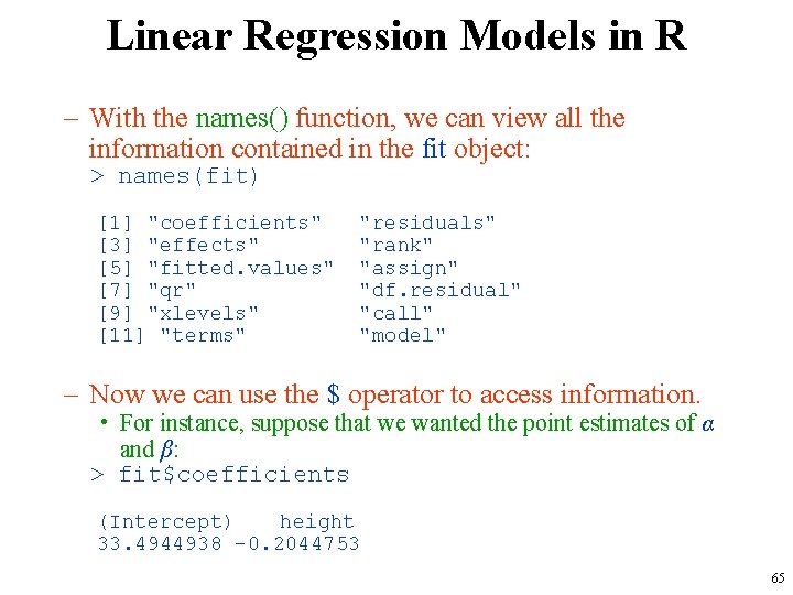
Linear Regression Models in R – With the names() function, we can view all the information contained in the fit object: > names(fit) [1] "coefficients" [3] "effects" [5] "fitted. values" [7] "qr" [9] "xlevels" [11] "terms" "residuals" "rank" "assign" "df. residual" "call" "model" – Now we can use the $ operator to access information. • For instance, suppose that we wanted the point estimates of α and β: > fit$coefficients (Intercept) height 33. 4944938 -0. 2044753 65

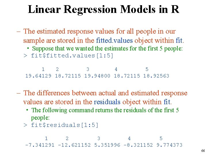
Linear Regression Models in R – The estimated response values for all people in our sample are stored in the fitted. values object within fit. • Suppose that we wanted the estimates for the first 5 people: > fit$fitted. values[1: 5] 1 2 3 4 5 19. 64129 18. 72115 19. 94800 18. 72115 18. 92563 – The differences between actual and estimated response values are stored in the residuals object within fit. • The following command returns the residuals of the first 5 people: > fit$residuals[1: 5] 1 2 3 4 5 -7. 341291 -12. 621152 5. 351996 -8. 321152 9. 774373 66

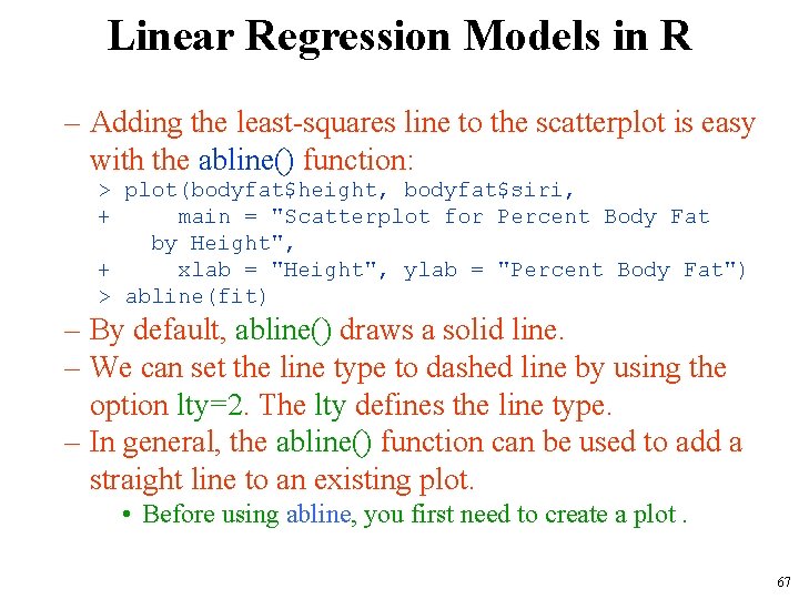
Linear Regression Models in R – Adding the least-squares line to the scatterplot is easy with the abline() function: > plot(bodyfat$height, bodyfat$siri, + main = "Scatterplot for Percent Body Fat by Height", + xlab = "Height", ylab = "Percent Body Fat") > abline(fit) – By default, abline() draws a solid line. – We can set the line type to dashed line by using the option lty=2. The lty defines the line type. – In general, the abline() function can be used to add a straight line to an existing plot. • Before using abline, you first need to create a plot. 67

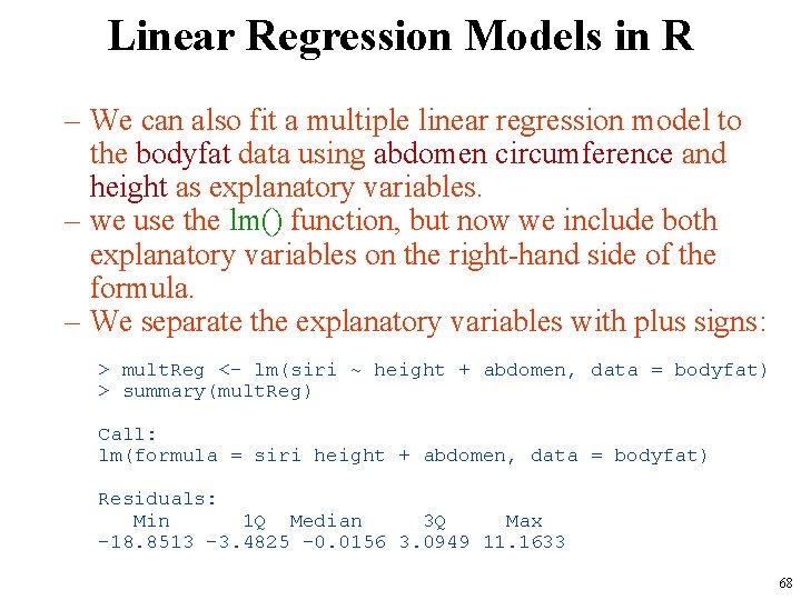
Linear Regression Models in R – We can also fit a multiple linear regression model to the bodyfat data using abdomen circumference and height as explanatory variables. – we use the lm() function, but now we include both explanatory variables on the right-hand side of the formula. – We separate the explanatory variables with plus signs: > mult. Reg <- lm(siri ~ height + abdomen, data = bodyfat) > summary(mult. Reg) Call: lm(formula = siri height + abdomen, data = bodyfat) Residuals: Min 1 Q Median 3 Q Max -18. 8513 -3. 4825 -0. 0156 3. 0949 11. 1633 68

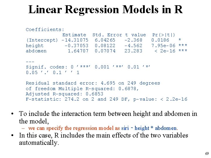
Linear Regression Models in R Coefficients: Estimate Std. Error (Intercept) -14. 31075 6. 04265 height -0. 37053 0. 08122 abdomen 1. 64707 0. 07074 t value -2. 368 -4. 562 23. 283 Pr(>|t|) 0. 0186 * 7. 95 e-06 *** < 2 e-16 *** --Signif. codes: 0 ’***’ 0. 001 ’**’ 0. 01 ’*’ 0. 05 ’. ’ 0. 1 ’ ’ 1 Residual standard error: 4. 695 on 249 degrees of freedom Multiple R-squared: 0. 6878, Adjusted R-squared: 0. 6853 F-statistic: 274. 2 on 2 and 249 DF, p-value: < 2. 2 e-16 • To include the interaction term between height and abdomen in the model, – we can specify the regression model as siri ∼ height * abdomen. • In this case, R includes the main effects of the two variables automatically. 69