Statistical Data Analysis Prof Dr Nizamettin AYDIN naydinyildiz

Statistical Data Analysis Prof. Dr. Nizamettin AYDIN naydin@yildiz. edu. tr http: //www 3. yildiz. edu. tr/~naydin 1

Estimation 2

Parameter Estimation • The objective of statistics is to make inferences about a population based on information contained in a sample. • Populations are characterized by numerical descriptive measures called parameters. • Typical population parameters are the mean m, the median M, the standard deviation s, and a proportion p. • Most inferential problems can be formulated as an inference about one or more parameters of a population. 3

Parameter Estimation • Methods for making inferences about parameters fall into one of two categories: – estimate the value of the population parameter of interest – test a hypothesis about the value of the parameter • These two methods of statistical inference involve different procedures, and they answer two different questions about the parameter: – In estimating a population parameter, we are answering the question • “What is the value of the population parameter? ” – In testing a hypothesis, we are seeking an answer to the question • “Does the population parameter satisfy a specified condition? ” 4

Parameter Estimation • We discussed – using random variables to represent characteristics of a population • (e. g. , BMI, disease status). – some commonly used probability distributions for discrete and continuous random variables. • We are specifically interested in population mean and population variance of a random variable. – These quantities are unknown in general. • We refer to these unknown quantities as parameters. • Here, we use parameters μ and σ2 to denote the unknown population mean and variance respectively. – Note that for all the distributions we discussed previously, the population mean and variance of a random variable are related to the unknown parameters of probability distribution assumed for that random variable. • Indeed, for normal distributions N(μ, σ2), which are widely used in statistics, the population mean and variance are exactly the same parameters used to specify the distribution. 5

Parameter Estimation • In this lecture, we discuss statistical methods for parameter estimation. – Estimation refers to the process of guessing the unknown value of a parameter (e. g. , population mean) using the observed data. • For this, we will use an estimator, which is a statistic. – A statistic is a function of the observed data only. • Sometimes we only provide a single value as our estimate. – This is called point estimation. • Point estimates do not reflect our uncertainty when estimating a parameter. • We always remain uncertain regarding the true value of the parameter when we estimate it using a sample from the population. • To address this issue, we can present our estimates in terms of a range of possible values. – This is called interval estimation. 6

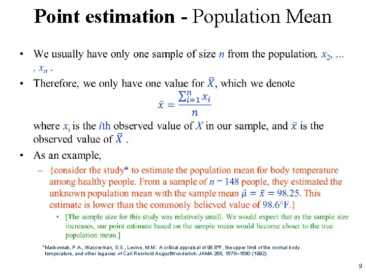
Convention • We use X 1, X 2, . . . , Xn to denote n possible values of X obtained from a sample randomly selected from the population. • We treat X 1, X 2, . . . , Xn themselves as n random variables because their values can change depending on which n individuals we sample. • We assume the samples are independent and identically distributed (IID). • While theoretically we can have many different samples of size n, we usually have only one such sample in practice. • We use x 1, x 2, . . . , xn as the specific set of values we have observed in our sample. • That is, x 1 is the observed value for X 1, x 2 is the observed value X 2, and so forth. 7

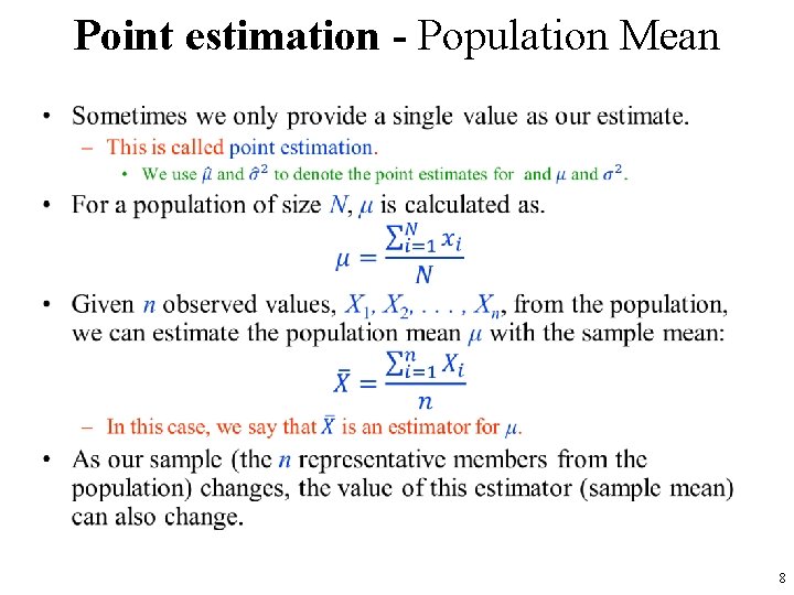
Point estimation - Population Mean • 8

Point estimation - Population Mean • *Mackowiak, P. A. , Wasserman, S. S. , Levine, M. M. : A critical appraisal of 98. 6°F, the upper limit of the normal body temperature, and other legacies of Carl Reinhold August. Wunderlich. JAMA 268, 1578– 1580 (1992) 9

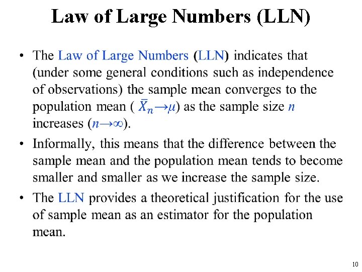
Law of Large Numbers (LLN) • 10

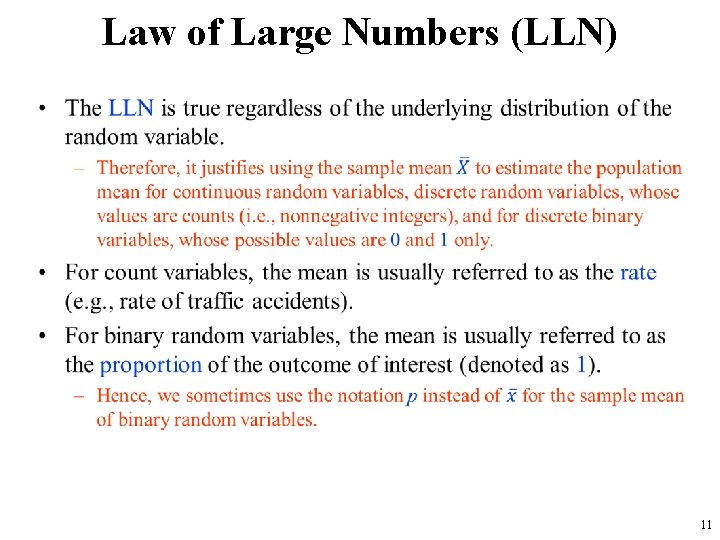
Law of Large Numbers (LLN) • 11

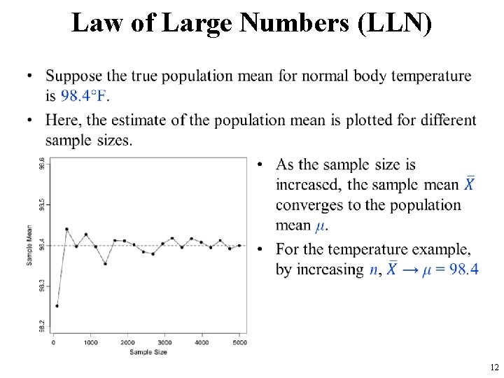
Law of Large Numbers (LLN) • 12

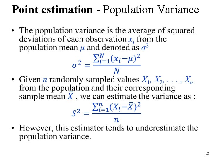
Point estimation - Population Variance • 13

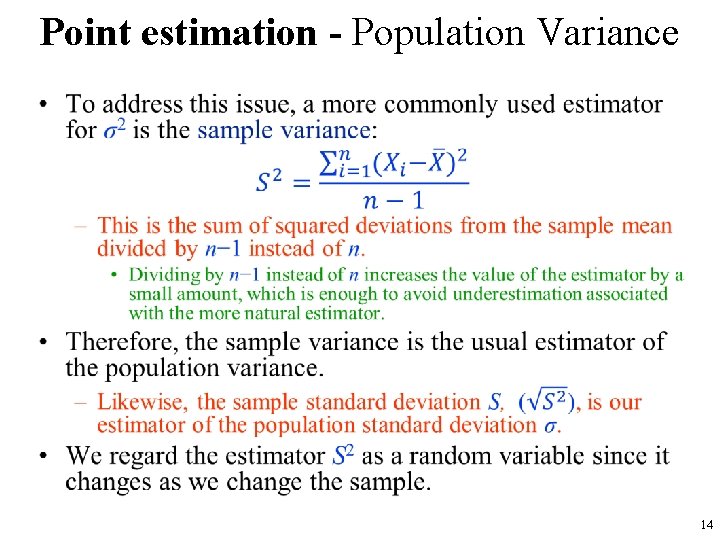
Point estimation - Population Variance • 14

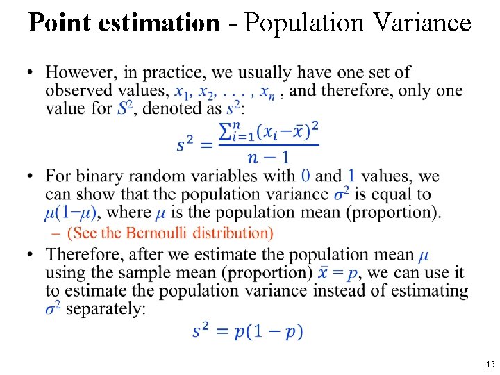
Point estimation - Population Variance • 15

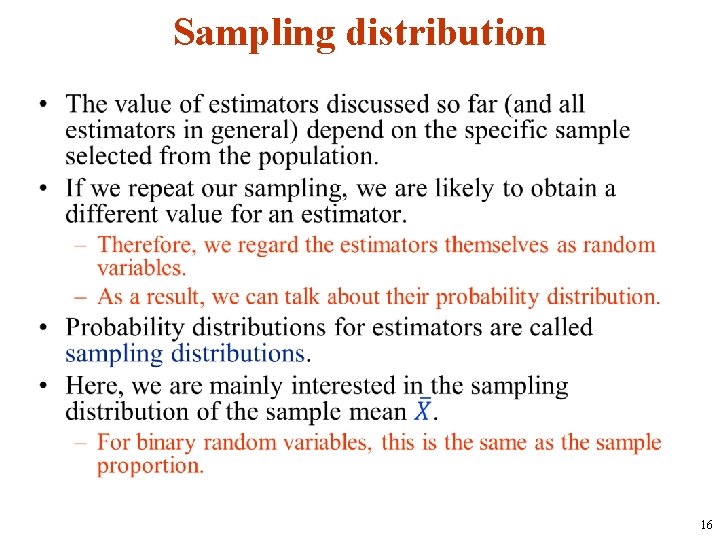
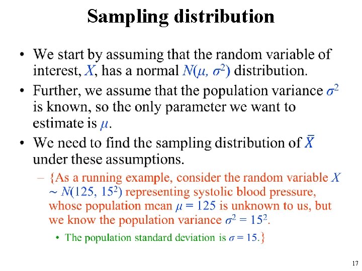
Sampling distribution • 16

Sampling distribution • 17

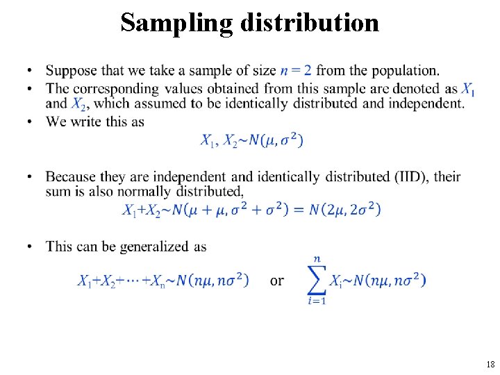
Sampling distribution • 18

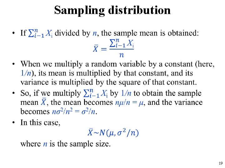
Sampling distribution • 19

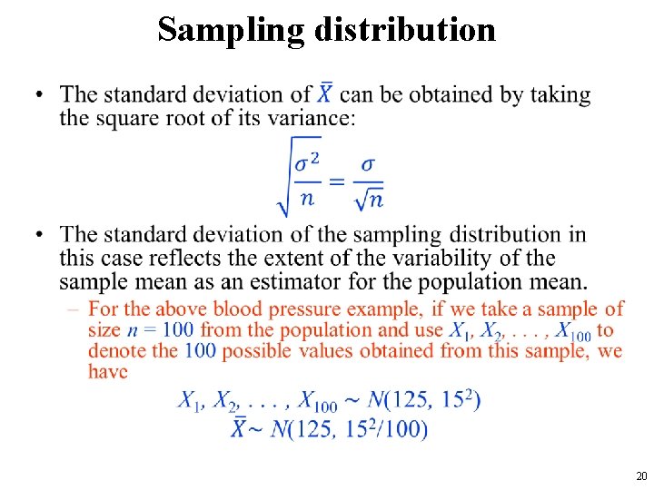
Sampling distribution • 20

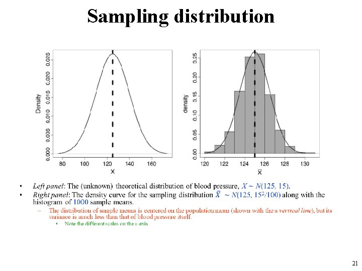
Sampling distribution • 21

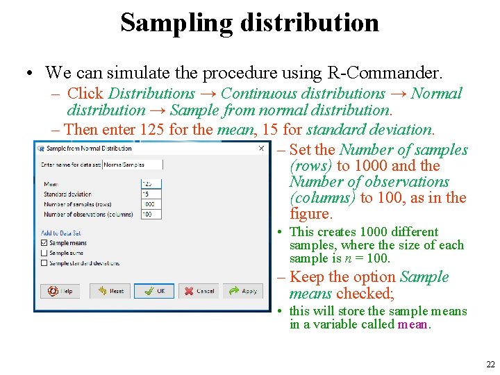
Sampling distribution • We can simulate the procedure using R-Commander. – Click Distributions → Continuous distributions → Normal distribution → Sample from normal distribution. – Then enter 125 for the mean, 15 for standard deviation. – Set the Number of samples (rows) to 1000 and the Number of observations (columns) to 100, as in the figure. • This creates 1000 different samples, where the size of each sample is n = 100. – Keep the option Sample means checked; • this will store the sample means in a variable called mean. 22

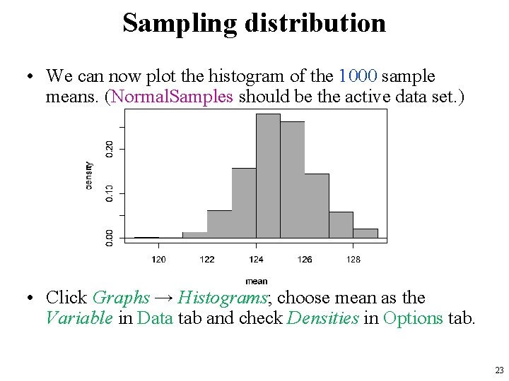
Sampling distribution • We can now plot the histogram of the 1000 sample means. (Normal. Samples should be the active data set. ) • Click Graphs → Histograms; choose mean as the Variable in Data tab and check Densities in Options tab. 23

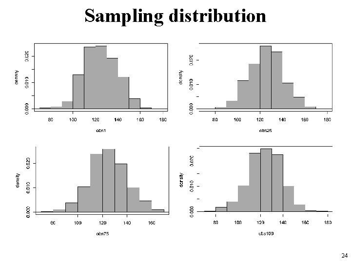
Sampling distribution 24

Confidence Intervals for the Population Mean • It is common to express our point estimate along with its standard deviation to show much the estimate could vary if different members of population were selected as our sample. • Alternatively, we can use the point estimate and its standard deviation to express our estimate as a range (interval) of possible values for the unknown parameter. 25

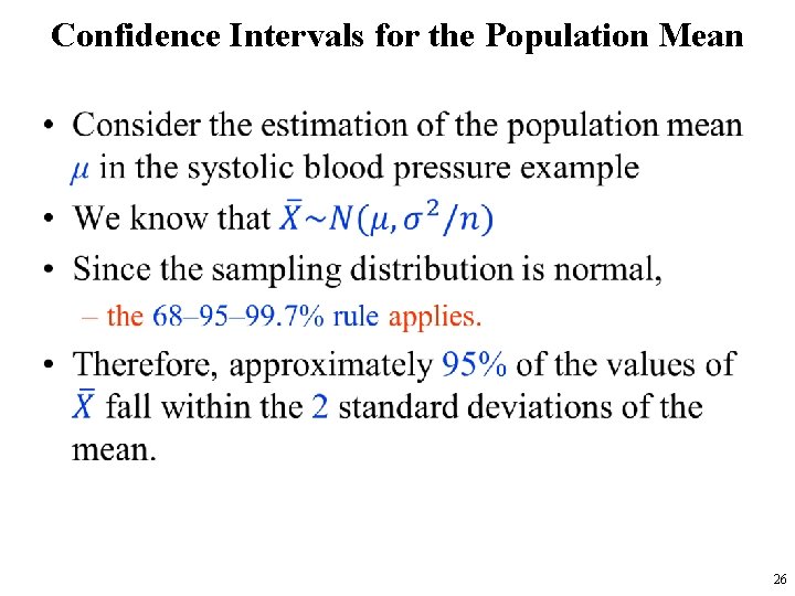
Confidence Intervals for the Population Mean • 26

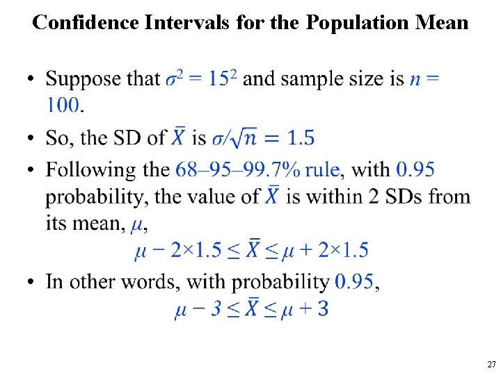
Confidence Intervals for the Population Mean • 27

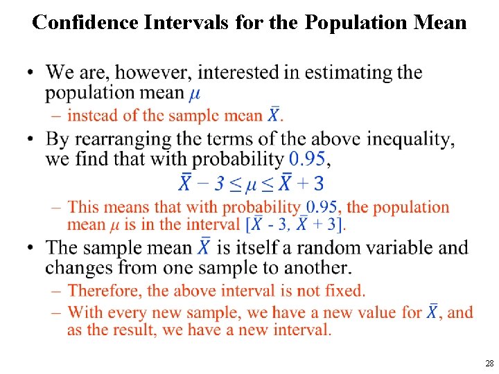
Confidence Intervals for the Population Mean • 28

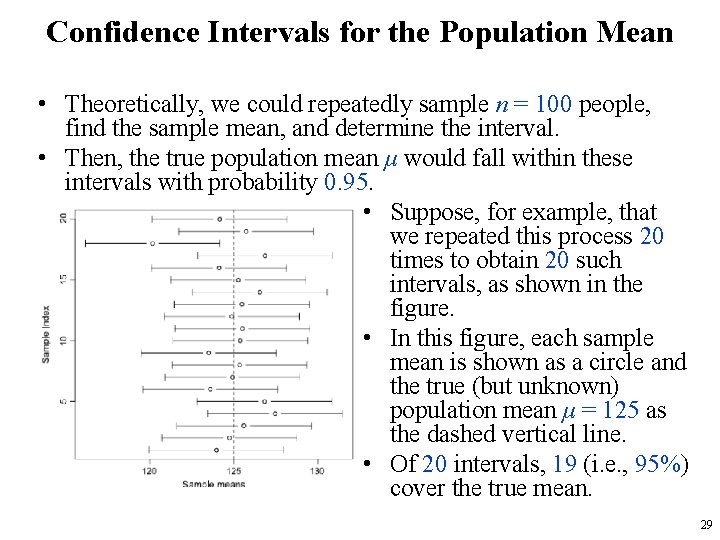
Confidence Intervals for the Population Mean • Theoretically, we could repeatedly sample n = 100 people, find the sample mean, and determine the interval. • Then, the true population mean μ would fall within these intervals with probability 0. 95. • Suppose, for example, that we repeated this process 20 times to obtain 20 such intervals, as shown in the figure. • In this figure, each sample mean is shown as a circle and the true (but unknown) population mean μ = 125 as the dashed vertical line. • Of 20 intervals, 19 (i. e. , 95%) cover the true mean. 29

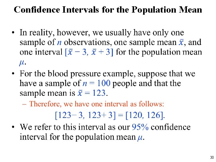
Confidence Intervals for the Population Mean • 30

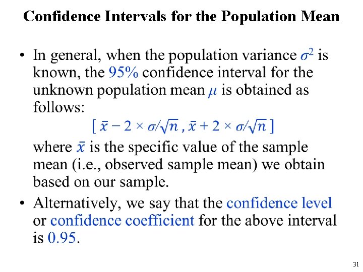
Confidence Intervals for the Population Mean • 31

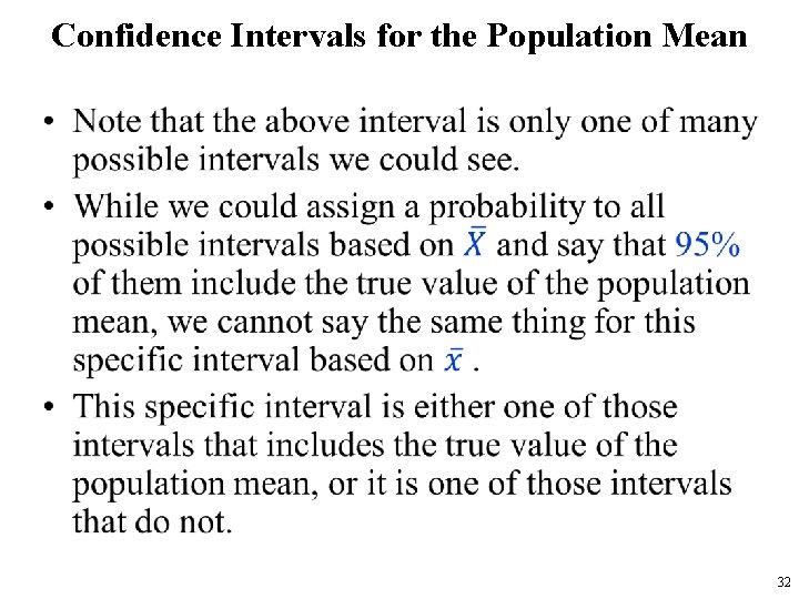
Confidence Intervals for the Population Mean • 32

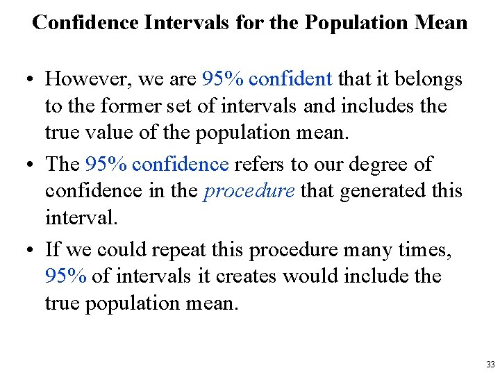
Confidence Intervals for the Population Mean • However, we are 95% confident that it belongs to the former set of intervals and includes the true value of the population mean. • The 95% confidence refers to our degree of confidence in the procedure that generated this interval. • If we could repeat this procedure many times, 95% of intervals it creates would include the true population mean. 33

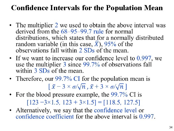
Confidence Intervals for the Population Mean • 34

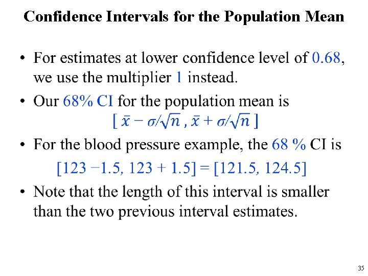
Confidence Intervals for the Population Mean • 35

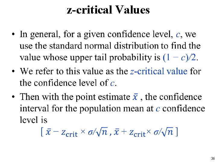
z-critical Values • 36

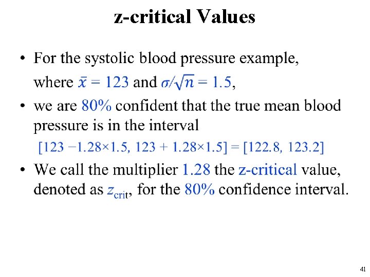
z-critical Values • Suppose that we want to set the confidence level of our interval estimate for the population mean to 0. 8. • To find the corresponding multiplier, we need to find the number of units we need to move from 0 on each side so that the probability of the resulting interval becomes 0. 8 based on the standard normal distribution. • The next figure shows the probability density curve of N(0, 1), which is known as the Z-curve. 37

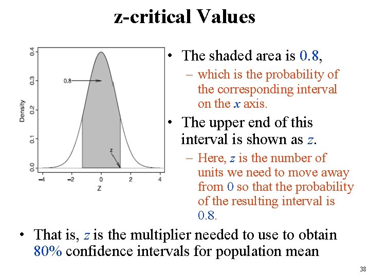
z-critical Values • The shaded area is 0. 8, – which is the probability of the corresponding interval on the x axis. • The upper end of this interval is shown as z. – Here, z is the number of units we need to move away from 0 so that the probability of the resulting interval is 0. 8. • That is, z is the multiplier needed to use to obtain 80% confidence intervals for population mean 38

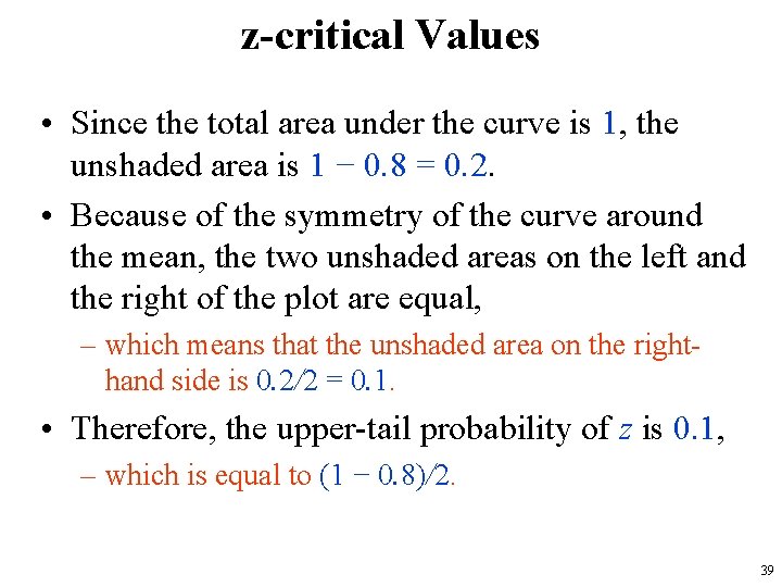
z-critical Values • Since the total area under the curve is 1, the unshaded area is 1 − 0. 8 = 0. 2. • Because of the symmetry of the curve around the mean, the two unshaded areas on the left and the right of the plot are equal, – which means that the unshaded area on the righthand side is 0. 2/2 = 0. 1. • Therefore, the upper-tail probability of z is 0. 1, – which is equal to (1 − 0. 8)/2. 39

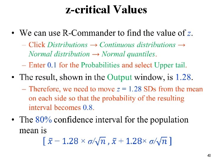
z-critical Values • 40

z-critical Values • 41

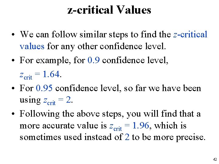
z-critical Values • We can follow similar steps to find the z-critical values for any other confidence level. • For example, for 0. 9 confidence level, zcrit = 1. 64. • For 0. 95 confidence level, so far we have been using zcrit = 2. • Following the above steps, you will find that a more accurate value is zcrit = 1. 96, which is sometimes used instead of 2 to be more precise. 42

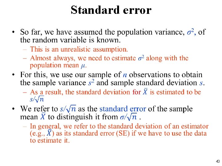
Standard error • 43

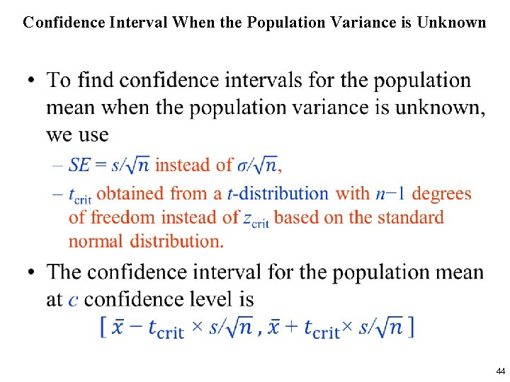
Confidence Interval When the Population Variance is Unknown • 44

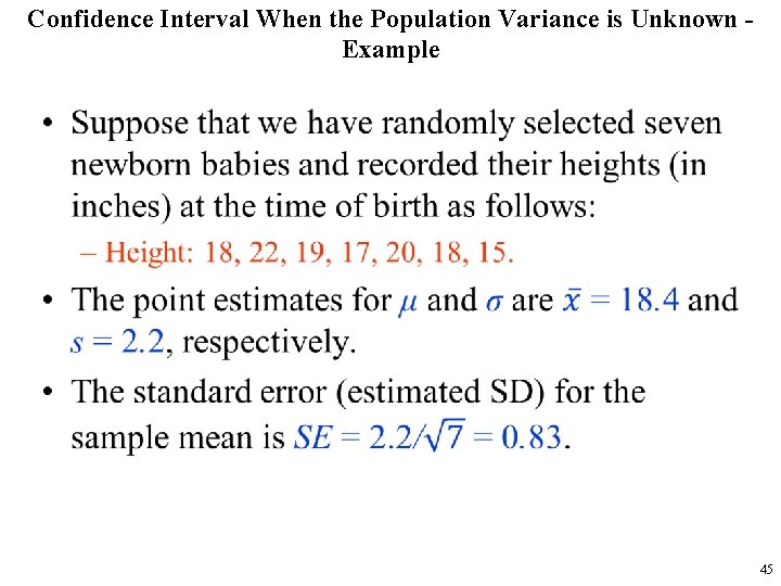
Confidence Interval When the Population Variance is Unknown Example • 45

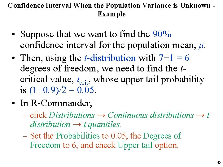
Confidence Interval When the Population Variance is Unknown Example • Suppose that we want to find the 90% confidence interval for the population mean, μ. • Then, using the t-distribution with 7− 1 = 6 degrees of freedom, we need to find the tcritical value, tcrit, whose upper tail probability is (1− 0. 9)/2 = 0. 05. • In R-Commander, – click Distributions → Continuous distributions → t distribution → t quantiles. – Set the Probabilities to 0. 05, the Degrees of Freedom to 6, and check Upper tail option. 46

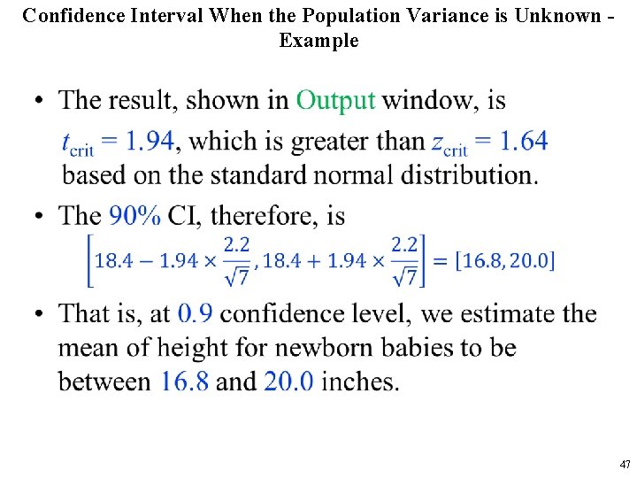
Confidence Interval When the Population Variance is Unknown Example • 47

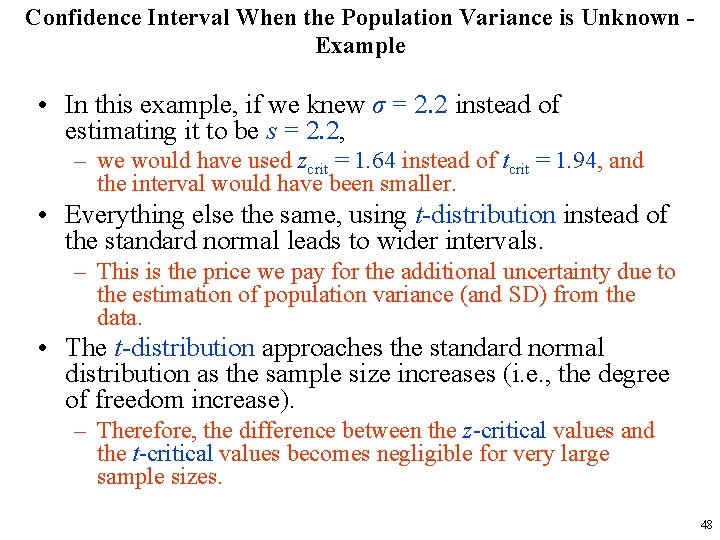
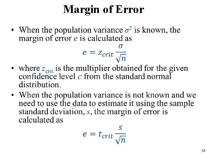
Confidence Interval When the Population Variance is Unknown Example • In this example, if we knew σ = 2. 2 instead of estimating it to be s = 2. 2, – we would have used zcrit = 1. 64 instead of tcrit = 1. 94, and the interval would have been smaller. • Everything else the same, using t-distribution instead of the standard normal leads to wider intervals. – This is the price we pay for the additional uncertainty due to the estimation of population variance (and SD) from the data. • The t-distribution approaches the standard normal distribution as the sample size increases (i. e. , the degree of freedom increase). – Therefore, the difference between the z-critical values and the t-critical values becomes negligible for very large sample sizes. 48

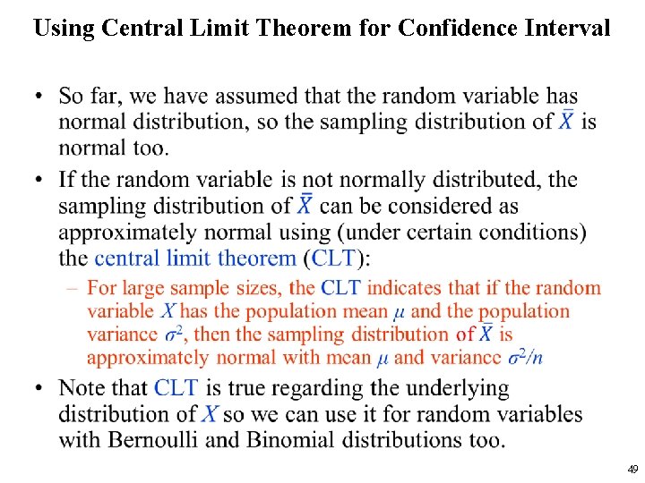
Using Central Limit Theorem for Confidence Interval • 49

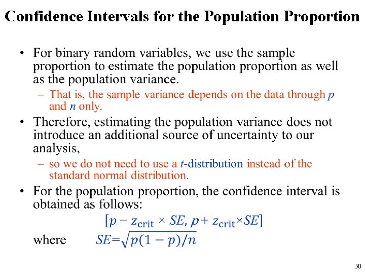
Confidence Intervals for the Population Proportion • 50

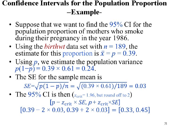
Confidence Intervals for the Population Proportion –Example- • 51

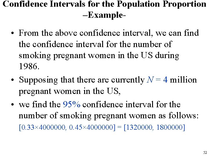
Confidence Intervals for the Population Proportion –Example- • From the above confidence interval, we can find the confidence interval for the number of smoking pregnant women in the US during 1986. • Supposing that there are currently N = 4 million pregnant women in the US, • we find the 95% confidence interval for the number of smoking pregnant women as follows: [0. 33× 4000000, 0. 45× 4000000] = [1320000, 1800000] 52

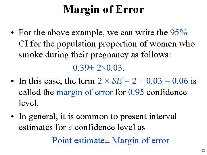
Margin of Error • For the above example, we can write the 95% CI for the population proportion of women who smoke during their pregnancy as follows: 0. 39± 2× 0. 03. • In this case, the term 2 × SE = 2 × 0. 03 = 0. 06 is called the margin of error for 0. 95 confidence level. • In general, it is common to present interval estimates for c confidence level as Point estimate± Margin of error 53

Margin of Error • 54

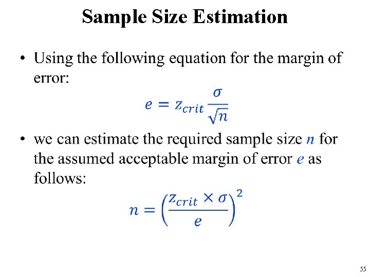
Sample Size Estimation • 55

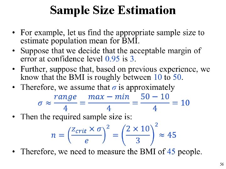
Sample Size Estimation • 56