Statistical Data Analysis Prof Dr Nizamettin AYDIN naydinyildiz

Statistical Data Analysis Prof. Dr. Nizamettin AYDIN naydin@yildiz. edu. tr http: //www. yildiz. edu. tr/~naydin 1

Examples 2

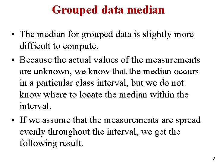
Grouped data median • The median for grouped data is slightly more difficult to compute. • Because the actual values of the measurements are unknown, we know that the median occurs in a particular class interval, but we do not know where to locate the median within the interval. • If we assume that the measurements are spread evenly throughout the interval, we get the following result. 3

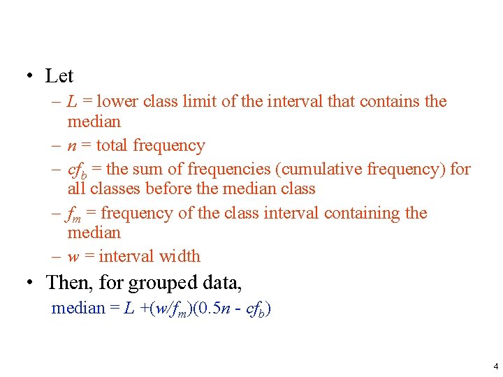
• Let – L = lower class limit of the interval that contains the median – n = total frequency – cfb = the sum of frequencies (cumulative frequency) for all classes before the median class – fm = frequency of the class interval containing the median – w = interval width • Then, for grouped data, median = L +(w/fm)(0. 5 n - cfb) 4

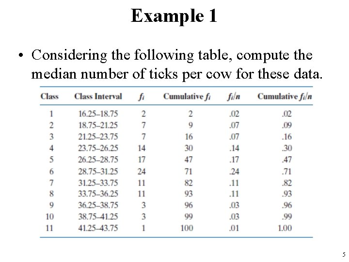
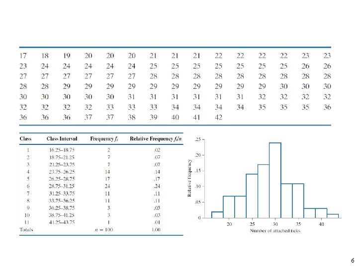
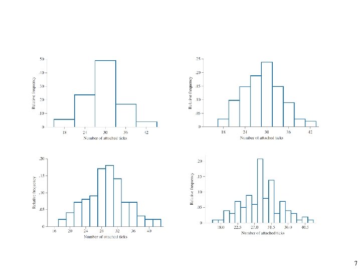
Example 1 • Considering the following table, compute the median number of ticks per cow for these data. 5

6

7

• Let the cumulative relative frequency for class j equal the sum of the relative frequencies for class 1 through class j. • To determine the interval that contains the median, we must find the first interval for which the cumulative relative frequency exceeds 0. 50. • This interval is the one containing the median. • For these data, the interval from 28. 75 to 31. 25 is the first interval for which the cumulative relative frequency exceeds 0. 50, as shown in table, Class 6. • So this interval contains the median. 8

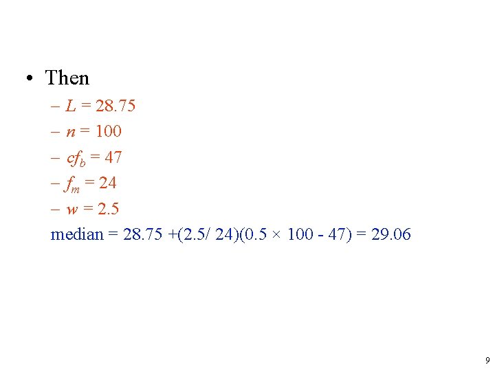
• Then – L = 28. 75 – n = 100 – cfb = 47 – fm = 24 – w = 2. 5 median = 28. 75 +(2. 5/ 24)(0. 5 × 100 - 47) = 29. 06 9

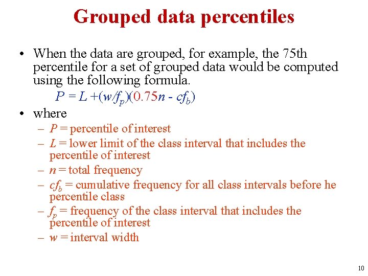
Grouped data percentiles • When the data are grouped, for example, the 75 th percentile for a set of grouped data would be computed using the following formula. P = L +(w/fp)(0. 75 n - cfb) • where – P = percentile of interest – L = lower limit of the class interval that includes the percentile of interest – n = total frequency – cfb = cumulative frequency for all class intervals before he percentile class – fp = frequency of the class interval that includes the percentile of interest – w = interval width 10

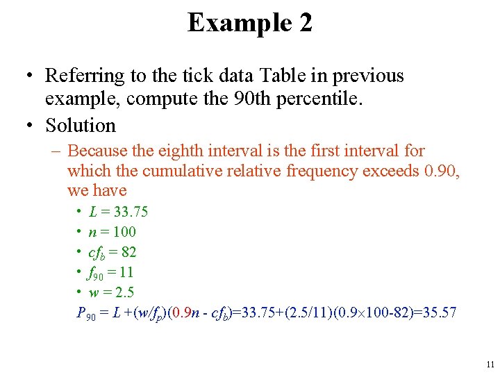
Example 2 • Referring to the tick data Table in previous example, compute the 90 th percentile. • Solution – Because the eighth interval is the first interval for which the cumulative relative frequency exceeds 0. 90, we have • L = 33. 75 • n = 100 • cfb = 82 • f 90 = 11 • w = 2. 5 P 90 = L +(w/fp)(0. 9 n - cfb)=33. 75+(2. 5/11)(0. 9 100 -82)=35. 57 11

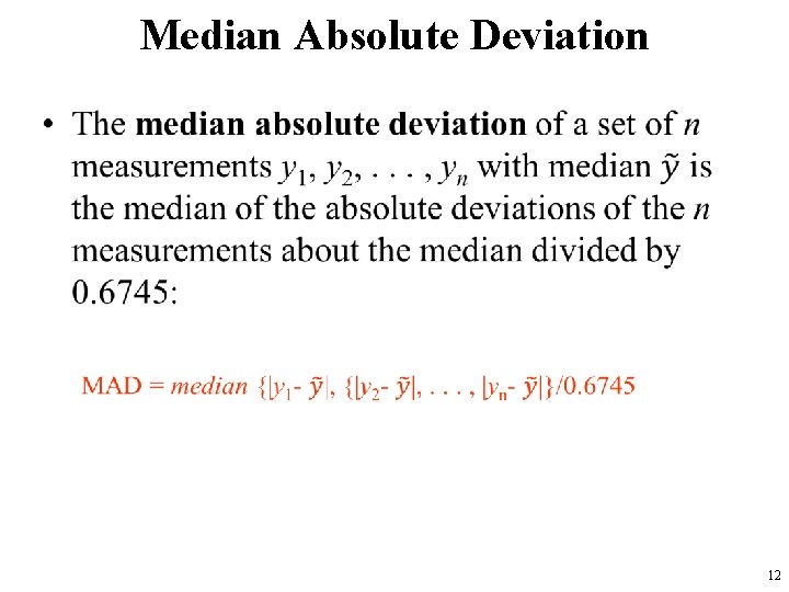
Median Absolute Deviation • 12

Median Absolute Deviation You may wonder why the median of the absolute deviations is divided by the value 0. 6745. In a population having a normal distribution with standard deviation s, the expected value of the absolute deviation about the median is 0. 6745 s. By dividing the median absolute deviation by 0. 6745, the expected value of MAD in a population having a normal distribution is equal to s. Thus, the values computed for MAD and the sample standard deviation are also the expected values for data randomly selected from populations that have a normal distribution. 13

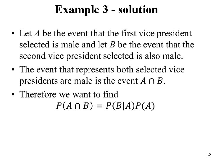
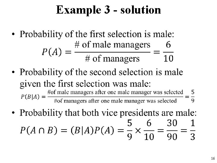
Example 3 • A corporation is proposing to select two of its current regional managers as vice presidents. In the history of the company, there has never been a female vice president. The corporation has six male regional managers and four female regional managers. Make the assumption that the 10 regional managers are equally qualified and hence all possible groups of two managers should have the same chance of being selected as the vice presidents. • Now find the probability that both vice presidents are male. 14

Example 3 - solution • 15

Example 3 - solution • 16

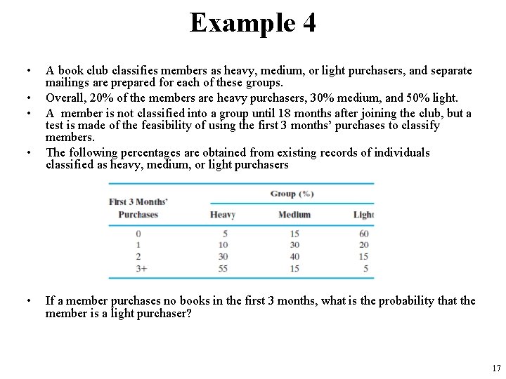
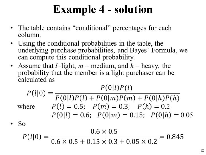
Example 4 • • • A book club classifies members as heavy, medium, or light purchasers, and separate mailings are prepared for each of these groups. Overall, 20% of the members are heavy purchasers, 30% medium, and 50% light. A member is not classified into a group until 18 months after joining the club, but a test is made of the feasibility of using the first 3 months’ purchases to classify members. The following percentages are obtained from existing records of individuals classified as heavy, medium, or light purchasers If a member purchases no books in the first 3 months, what is the probability that the member is a light purchaser? 17

Example 4 - solution • 18

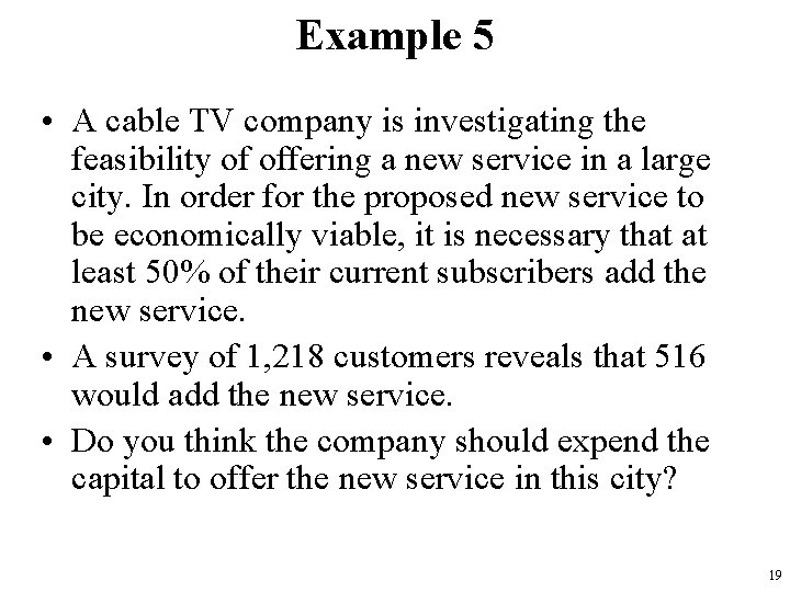
Example 5 • A cable TV company is investigating the feasibility of offering a new service in a large city. In order for the proposed new service to be economically viable, it is necessary that at least 50% of their current subscribers add the new service. • A survey of 1, 218 customers reveals that 516 would add the new service. • Do you think the company should expend the capital to offer the new service in this city? 19

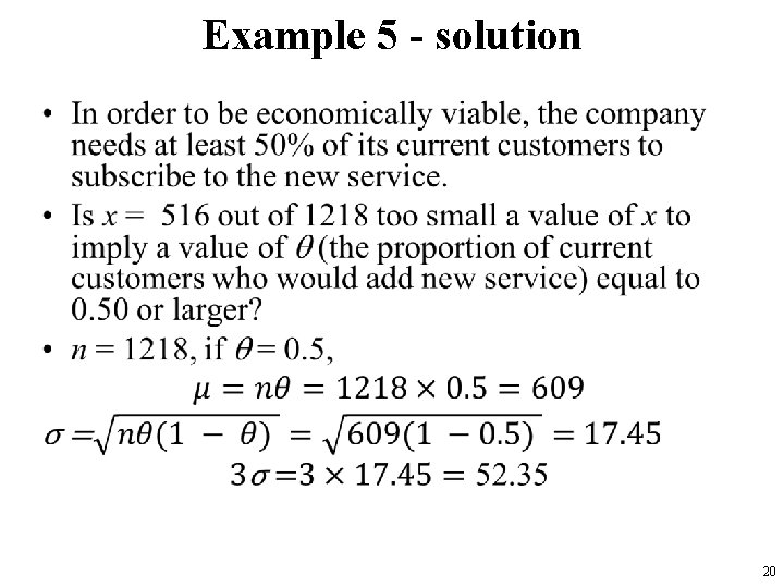
Example 5 - solution • 20

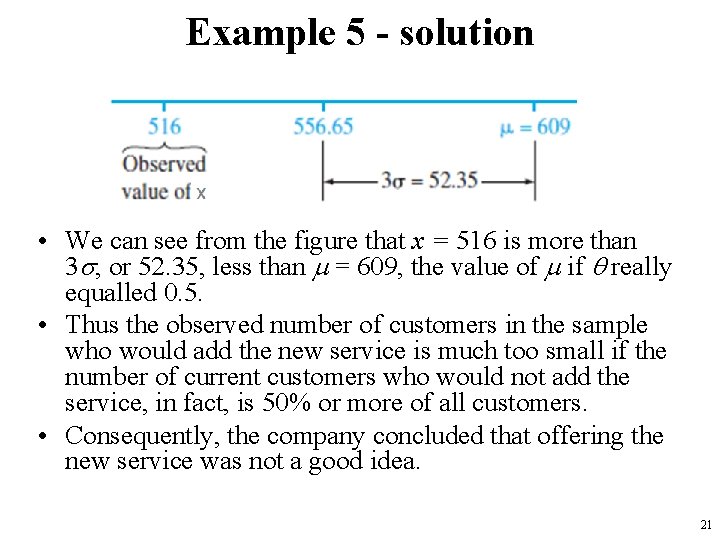
Example 5 - solution • We can see from the figure that x = 516 is more than 3 s, or 52. 35, less than m = 609, the value of m if really equalled 0. 5. • Thus the observed number of customers in the sample who would add the new service is much too small if the number of current customers who would not add the service, in fact, is 50% or more of all customers. • Consequently, the company concluded that offering the new service was not a good idea. 21

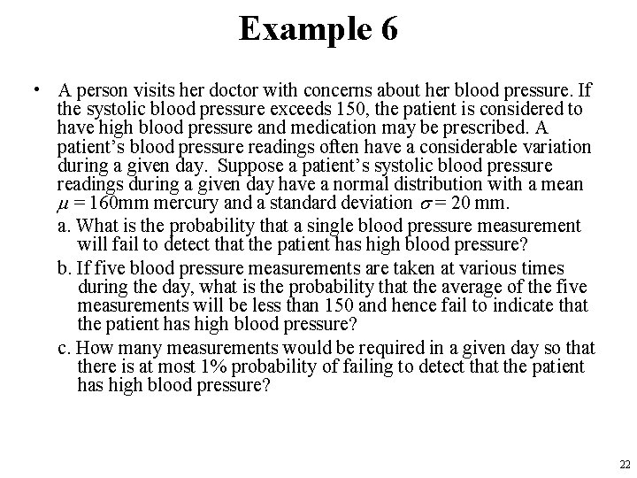
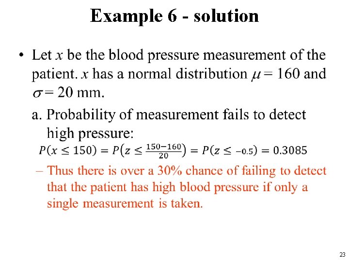
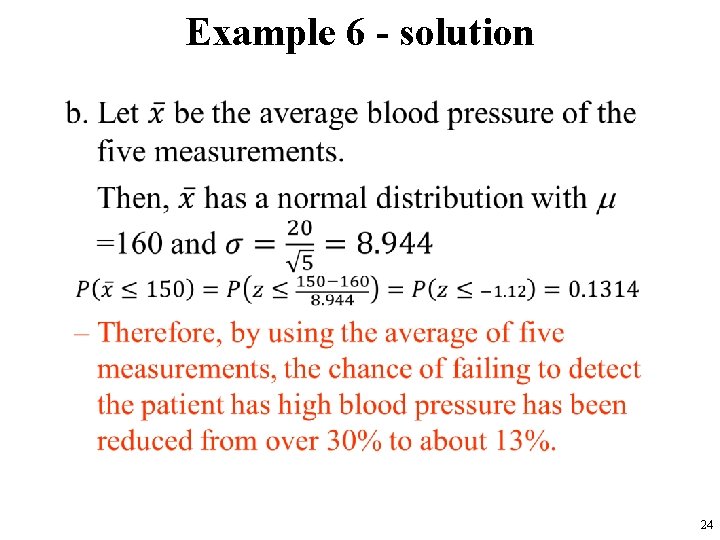
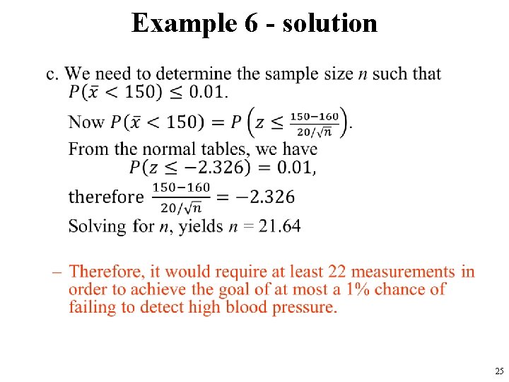
Example 6 • A person visits her doctor with concerns about her blood pressure. If the systolic blood pressure exceeds 150, the patient is considered to have high blood pressure and medication may be prescribed. A patient’s blood pressure readings often have a considerable variation during a given day. Suppose a patient’s systolic blood pressure readings during a given day have a normal distribution with a mean m = 160 mm mercury and a standard deviation s = 20 mm. a. What is the probability that a single blood pressure measurement will fail to detect that the patient has high blood pressure? b. If five blood pressure measurements are taken at various times during the day, what is the probability that the average of the five measurements will be less than 150 and hence fail to indicate that the patient has high blood pressure? c. How many measurements would be required in a given day so that there is at most 1% probability of failing to detect that the patient has high blood pressure? 22

Example 6 - solution • 23

Example 6 - solution • 24

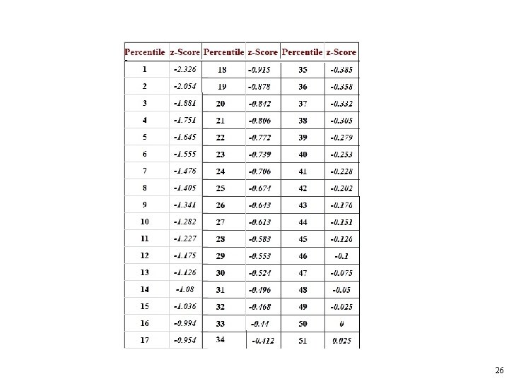
Example 6 - solution • 25

26

27

28

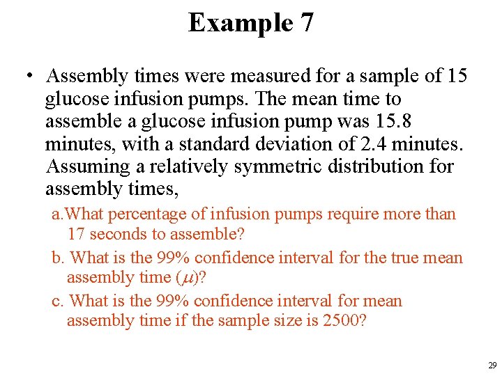
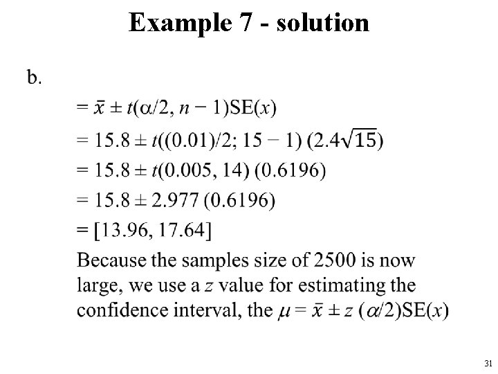
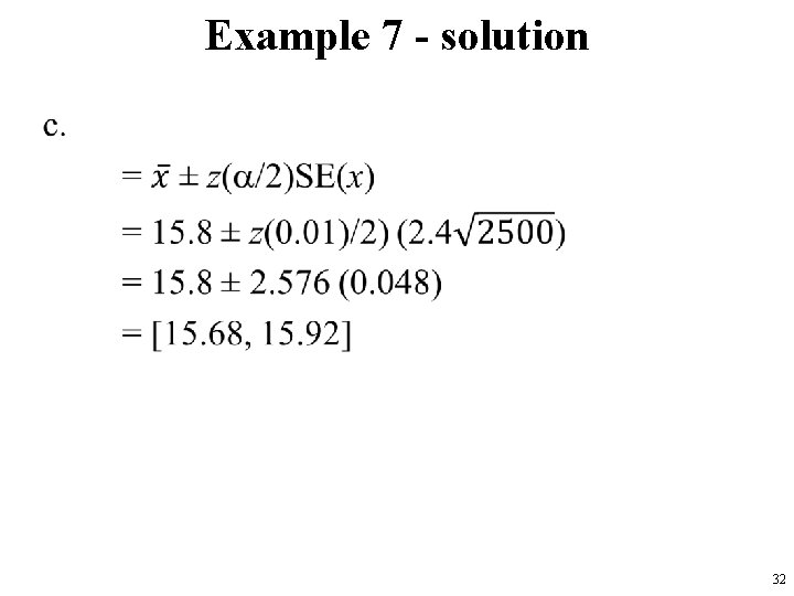
Example 7 • Assembly times were measured for a sample of 15 glucose infusion pumps. The mean time to assemble a glucose infusion pump was 15. 8 minutes, with a standard deviation of 2. 4 minutes. Assuming a relatively symmetric distribution for assembly times, a. What percentage of infusion pumps require more than 17 seconds to assemble? b. What is the 99% confidence interval for the true mean assembly time (m)? c. What is the 99% confidence interval for mean assembly time if the sample size is 2500? 29

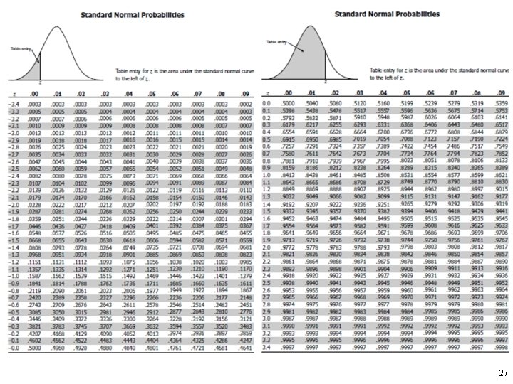
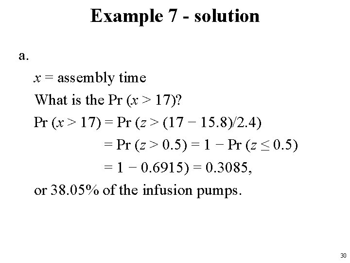
Example 7 - solution a. x = assembly time What is the Pr (x > 17)? Pr (x > 17) = Pr (z > (17 − 15. 8)/2. 4) = Pr (z > 0. 5) = 1 − Pr (z ≤ 0. 5) = 1 − 0. 6915) = 0. 3085, or 38. 05% of the infusion pumps. 30

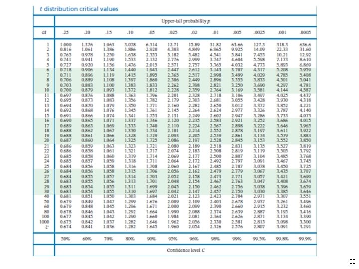
Example 7 - solution • 31

Example 7 - solution • 32