Statistical Data Analysis Prof Dr Nizamettin AYDIN naydinyildiz

Statistical Data Analysis Prof. Dr. Nizamettin AYDIN naydin@yildiz. edu. tr http: //www 3. yildiz. edu. tr/~naydin 1

Bayesian Analysis 2

Bayesian inference • Bayes’ theorem is the basis of the Bayesian Statistics. • It describes the probability of an event, based on prior knowledge of conditions that might be related to the event – For example, if the risk of developing health problems is known to increase with age, Bayes' theorem allows the risk to an individual of a known age to be assessed more accurately (by conditioning it on their age) than simply assuming that the individual is typical of the population as a whole. • Bayesian inference regarding the population proportion – an example for the application of Bayesian methods. 3

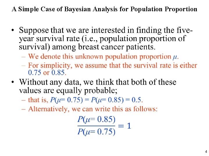
A Simple Case of Bayesian Analysis for Population Proportion • 4

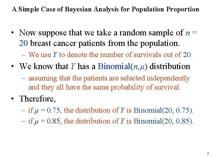
A Simple Case of Bayesian Analysis for Population Proportion • Now suppose that we take a random sample of n = 20 breast cancer patients from the population. – We use Y to denote the number of survivals out of 20. • We know that Y has a Binomial(n, μ) distribution – assuming that the patients are selected independently and they all have the same probability of survival. • Therefore, – if μ = 0. 75, the distribution of Y is Binomial(20, 0. 75). – if μ = 0. 85, the distribution of Y is Binomial(20, 0. 85). 5

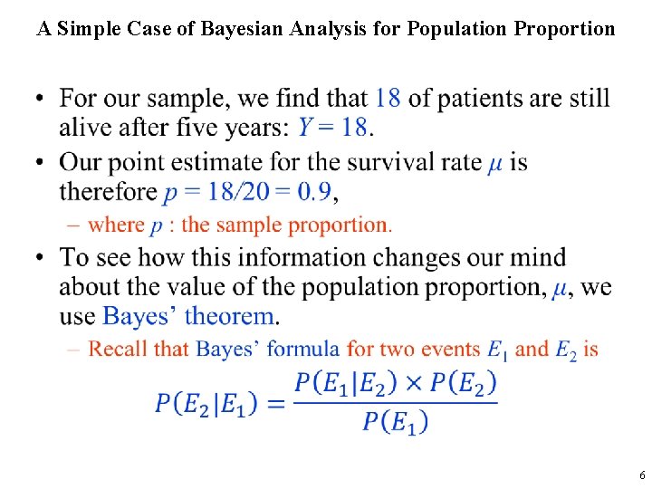
A Simple Case of Bayesian Analysis for Population Proportion • 6

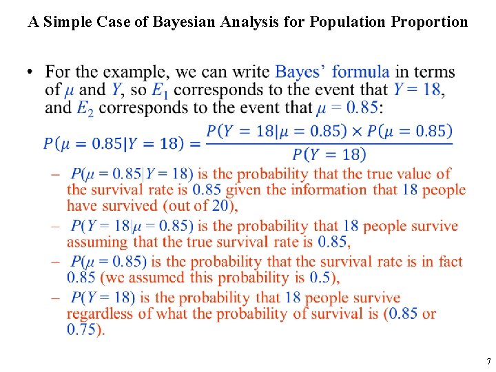
A Simple Case of Bayesian Analysis for Population Proportion • 7

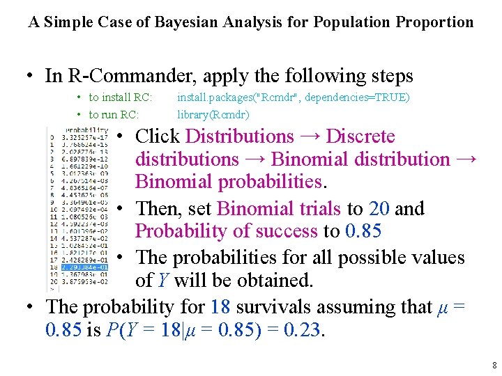
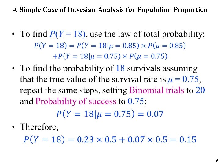
A Simple Case of Bayesian Analysis for Population Proportion • In R-Commander, apply the following steps • to install RC: • to run RC: install. packages("Rcmdr", dependencies=TRUE) library(Rcmdr) • Click Distributions → Discrete distributions → Binomial distribution → Binomial probabilities. • Then, set Binomial trials to 20 and Probability of success to 0. 85 • The probabilities for all possible values of Y will be obtained. • The probability for 18 survivals assuming that μ = 0. 85 is P(Y = 18|μ = 0. 85) = 0. 23. 8

A Simple Case of Bayesian Analysis for Population Proportion • 9

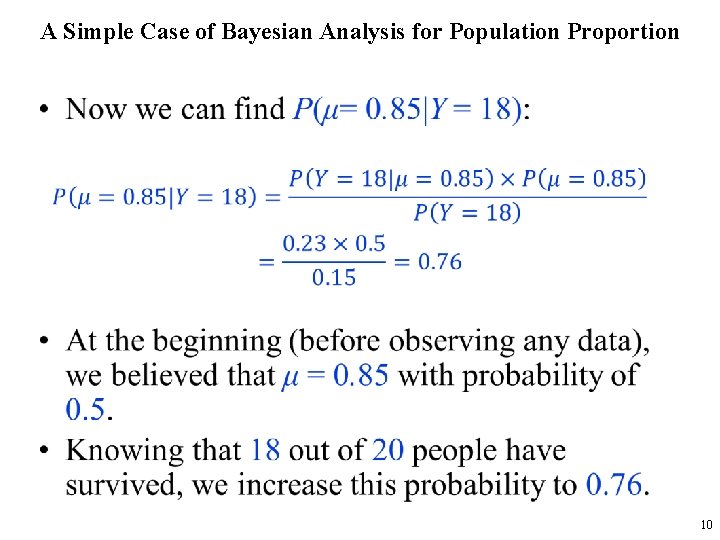
A Simple Case of Bayesian Analysis for Population Proportion • 10

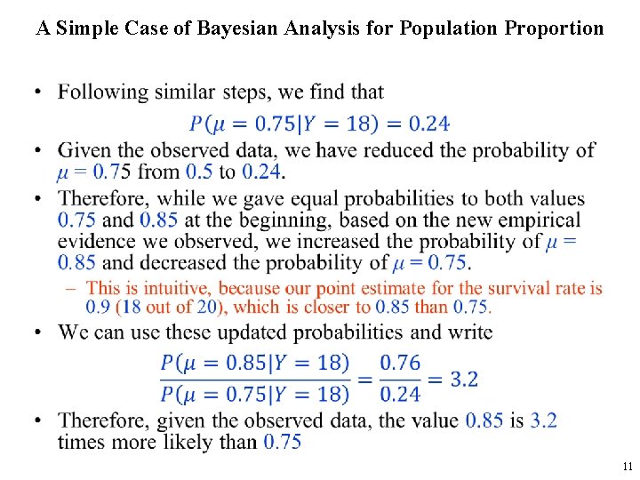
A Simple Case of Bayesian Analysis for Population Proportion • 11

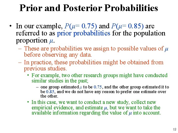
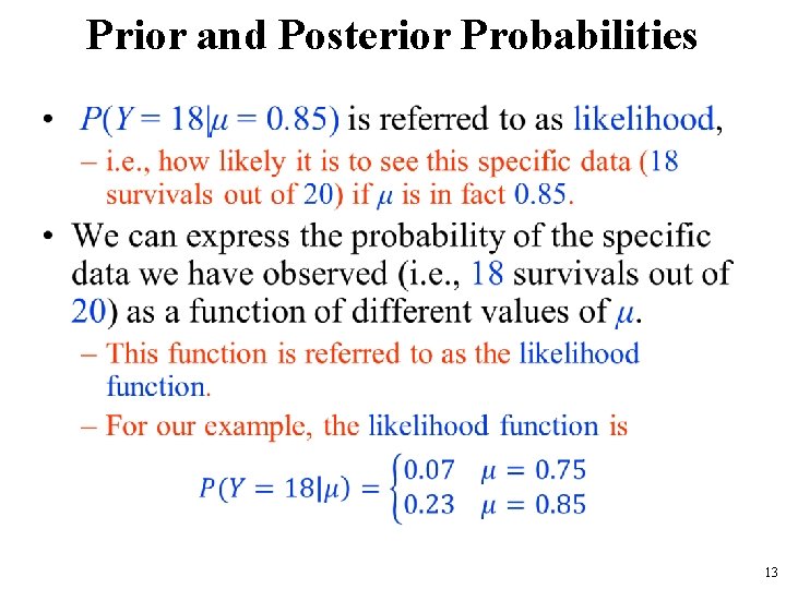
Prior and Posterior Probabilities • In our example, P(μ= 0. 75) and P(μ= 0. 85) are referred to as prior probabilities for the population proportion μ. – These are probabilities we assign to possible values of μ before observing any data. – In practice, these probabilities might be obtained from previous studies. • For example, two other research groups might have conducted similar studies in the past; – one group estimated μ to be 0. 75, and the other group estimated it to be 0. 85, and we do not have any reason to prefer one estimate over the other. • In this case, we want to conduct a new study, collect new empirical evidence, and estimate μ, but we want to take the available information regarding the value of μ into account. 12

Prior and Posterior Probabilities • 13

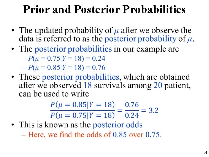
Prior and Posterior Probabilities • 14

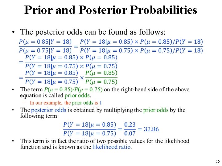
Prior and Posterior Probabilities • 15

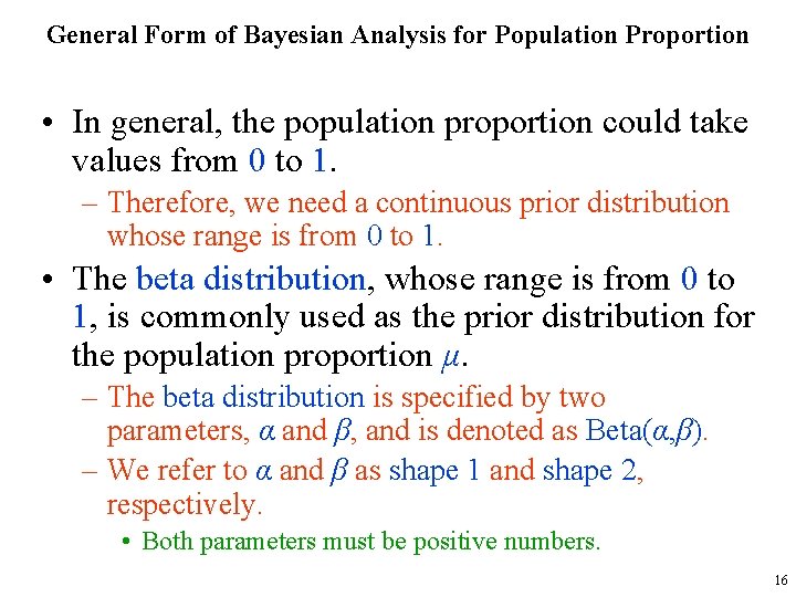
General Form of Bayesian Analysis for Population Proportion • In general, the population proportion could take values from 0 to 1. – Therefore, we need a continuous prior distribution whose range is from 0 to 1. • The beta distribution, whose range is from 0 to 1, is commonly used as the prior distribution for the population proportion μ. – The beta distribution is specified by two parameters, α and β, and is denoted as Beta(α, β). – We refer to α and β as shape 1 and shape 2, respectively. • Both parameters must be positive numbers. 16

General Form of Bayesian Analysis for Population Proportion • In R-Commander, we can plot different beta distributions by setting α and β to different values. • For example, suppose that we want to plot Beta(8, 2). • In R-Commander, click Distributions → Continuous distributions → Beta distribution → Plot beta distribution and set Shape 1 and Shape 2 to 8 and 2, respectively. • Make sure the option Plot density function is checked and press OK. 17

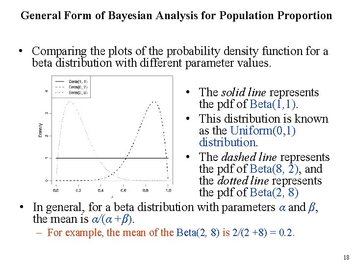
General Form of Bayesian Analysis for Population Proportion • Comparing the plots of the probability density function for a beta distribution with different parameter values. • The solid line represents the pdf of Beta(1, 1). • This distribution is known as the Uniform(0, 1) distribution. • The dashed line represents the pdf of Beta(8, 2), and the dotted line represents the pdf of Beta(2, 8) • In general, for a beta distribution with parameters α and β, the mean is α/(α +β). – For example, the mean of the Beta(2, 8) is 2/(2 +8) = 0. 2. 18

General Form of Bayesian Analysis for Population Proportion • Reconsider the breast cancer survival example. – Instead of assuming that only two values are possible, assume that the true population proportion could be any value from 0 to 1 • In general, it is recommended to avoid making overly restrictive assumptions such as the one we used for illustrative purposes earlier. – That is, even if previous studies estimated the population proportion to be either 0. 75 and 0. 85, we still should consider all other feasible values. 19

General Form of Bayesian Analysis for Population Proportion • We could of course use the results from previous studies and assume that while the survival rate could be any value from 0 to 1, it is more likely to be around 0. 8. • When specifying the prior distribution, we can use a beta distribution that reflects this assumption. – For the Beta(8, 2) distribution (dashed curve in the figure in slide 18), the probability (i. e. , the area under the density curve) is high for values around 0. 8, whereas the probability is almost zero for values around 0. 2. • Therefore, we use Beta(8, 2) as the prior distribution for the survival rate of breast cancer patients. 20

General Form of Bayesian Analysis for Population Proportion • Note that this prior probability distribution reflects our knowledge (based on previous studies) regarding the possible values of survival rate before we obtain new data. – We update our knowledge after we observe new empirical evidence. • Our updated knowledge is expressed as the posterior probability distribution, which could be drastically different from the prior probability distribution. – Therefore, even though we believe in prior that the survival rate is around 0. 8, a new empirical evidence could overwhelmingly change this belief. – We might be even convinced that values around 0. 2 are more probable than values around 0. 8 if the observed data strongly suggest that. 21

General Form of Bayesian Analysis for Population Proportion • To find the posterior probability (PP) distribution, we use Bayes’ theorem as before. – PP Distribution is a beta distribution with updated parameters • If we assume that the prior knowledge of the population proportion μ, can be expressed using a Beta(α, β) distribution, then the posterior distribution of μ is Beta(α +y, β+n−y), – where n is the sample size, and y is the number of times the event of interest has been observed. 22

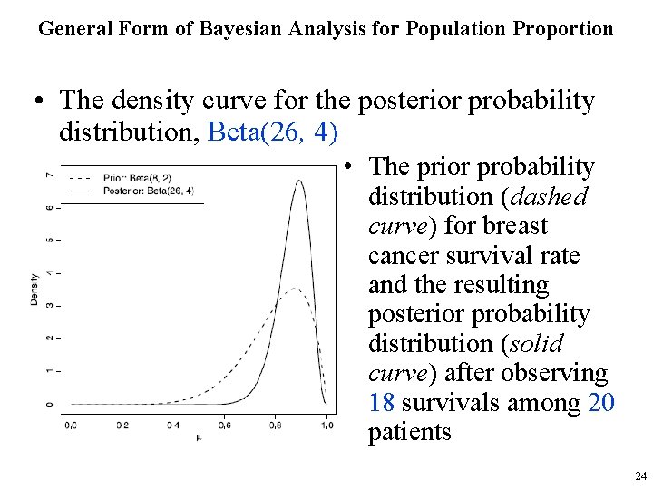
General Form of Bayesian Analysis for Population Proportion • In our example, we obtained a sample of 20 patients from the population and found that 18 of them survived after 5 years. • Assuming that the prior probability distribution for the breast cancer survival rate is Beta(8, 2), the posterior probability distribution for the survival rate is Beta(8+18, 2+20− 18). • We can use R-Commander to plot the probability density function for this distribution by following the steps described earlier, but this time we set Shape 1 and Shape 2 to 26 and 4, respectively. 23

General Form of Bayesian Analysis for Population Proportion • The density curve for the posterior probability distribution, Beta(26, 4) • The prior probability distribution (dashed curve) for breast cancer survival rate and the resulting posterior probability distribution (solid curve) after observing 18 survivals among 20 patients 24