Statistical Analysis using SPSS Dr Shaikh Shaffi Ahamed

Statistical Analysis using SPSS Dr. Shaikh Shaffi Ahamed Asst. Professor Dept. of Family & Community Medicine

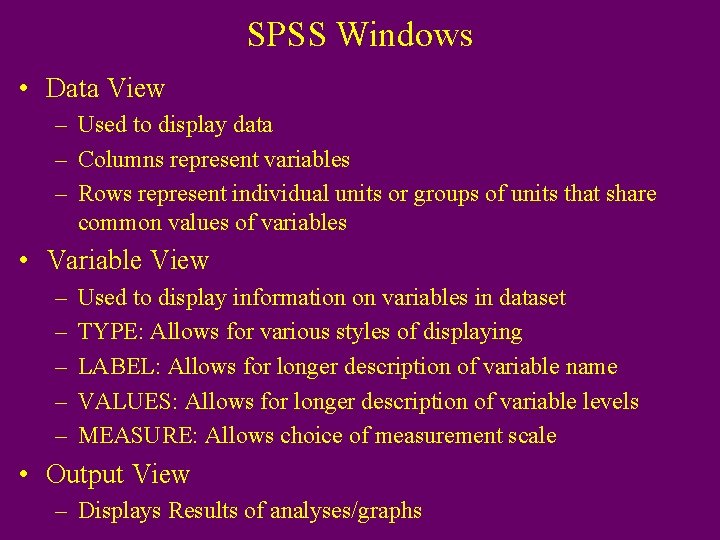
SPSS Windows • Data View – Used to display data – Columns represent variables – Rows represent individual units or groups of units that share common values of variables • Variable View – – – Used to display information on variables in dataset TYPE: Allows for various styles of displaying LABEL: Allows for longer description of variable name VALUES: Allows for longer description of variable levels MEASURE: Allows choice of measurement scale • Output View – Displays Results of analyses/graphs

Data Entry Tips • For large datasets, use a spreadsheet such as EXCEL which is more flexible for data entry, and import the file into SPSS • Give descriptive LABEL to variable names in the VARIABLE VIEW • Keep in mind that Columns are Variables, you don’t want multiple columns with the same variable

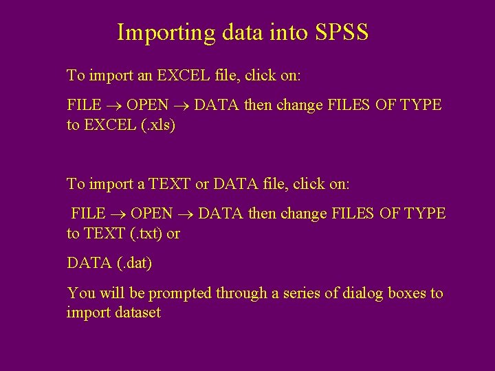
Importing data into SPSS To import an EXCEL file, click on: FILE OPEN DATA then change FILES OF TYPE to EXCEL (. xls) To import a TEXT or DATA file, click on: FILE OPEN DATA then change FILES OF TYPE to TEXT (. txt) or DATA (. dat) You will be prompted through a series of dialog boxes to import dataset

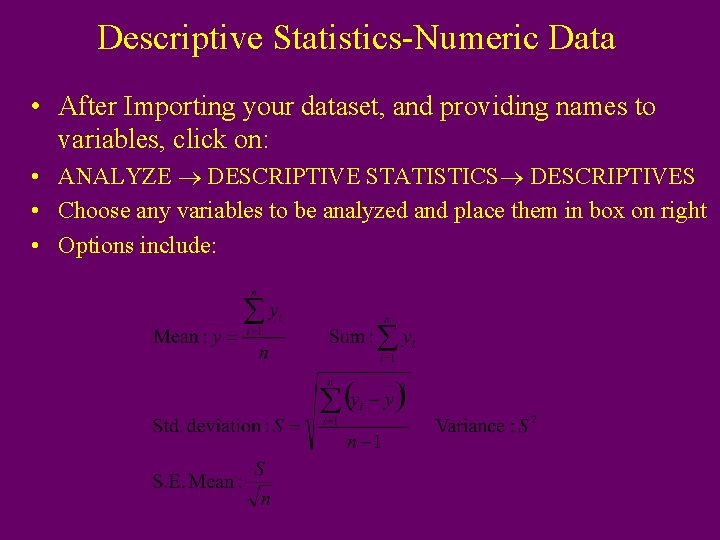
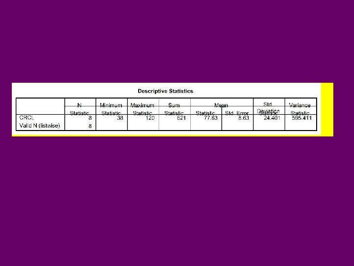
Descriptive Statistics-Numeric Data • After Importing your dataset, and providing names to variables, click on: • ANALYZE DESCRIPTIVE STATISTICS DESCRIPTIVES • Choose any variables to be analyzed and place them in box on right • Options include:

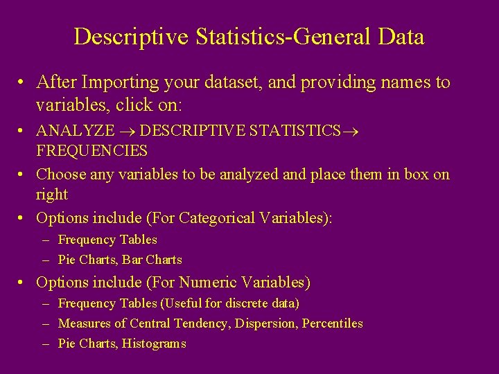
Descriptive Statistics-General Data • After Importing your dataset, and providing names to variables, click on: • ANALYZE DESCRIPTIVE STATISTICS FREQUENCIES • Choose any variables to be analyzed and place them in box on right • Options include (For Categorical Variables): – Frequency Tables – Pie Charts, Bar Charts • Options include (For Numeric Variables) – Frequency Tables (Useful for discrete data) – Measures of Central Tendency, Dispersion, Percentiles – Pie Charts, Histograms

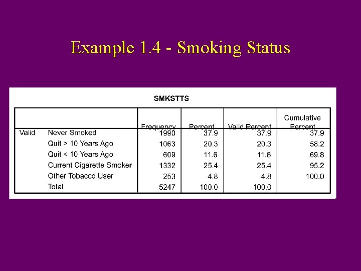
Example 1. 4 - Smoking Status

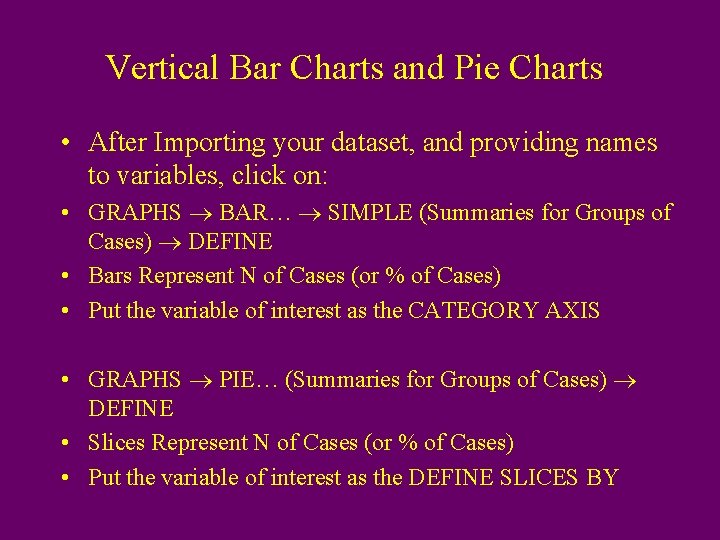
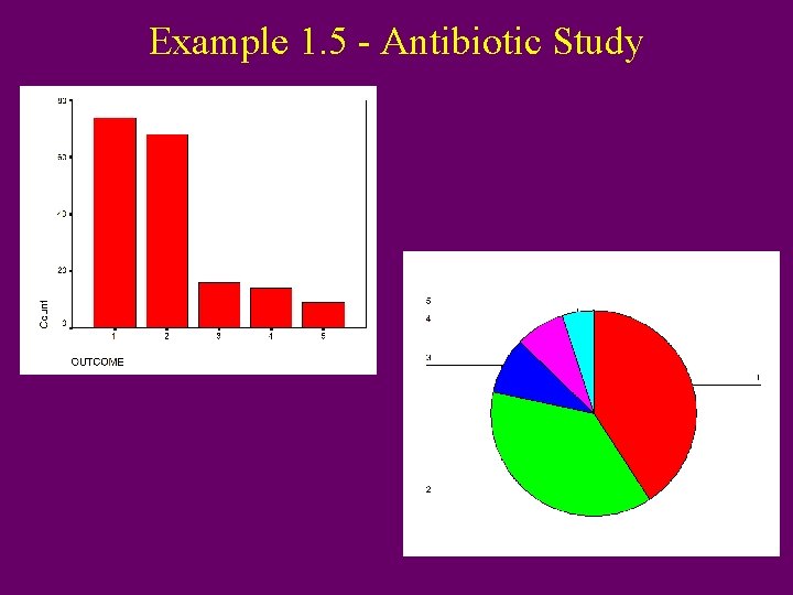
Vertical Bar Charts and Pie Charts • After Importing your dataset, and providing names to variables, click on: • GRAPHS BAR… SIMPLE (Summaries for Groups of Cases) DEFINE • Bars Represent N of Cases (or % of Cases) • Put the variable of interest as the CATEGORY AXIS • GRAPHS PIE… (Summaries for Groups of Cases) DEFINE • Slices Represent N of Cases (or % of Cases) • Put the variable of interest as the DEFINE SLICES BY

Example 1. 5 - Antibiotic Study

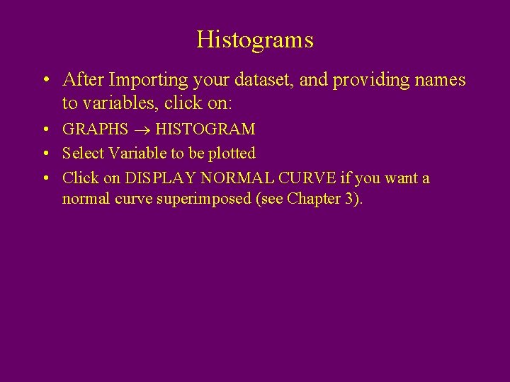
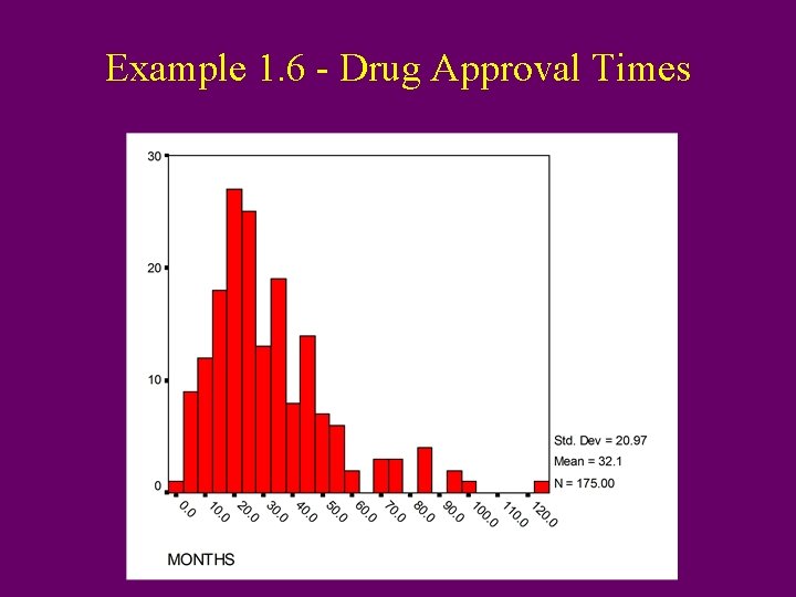
Histograms • After Importing your dataset, and providing names to variables, click on: • GRAPHS HISTOGRAM • Select Variable to be plotted • Click on DISPLAY NORMAL CURVE if you want a normal curve superimposed (see Chapter 3).

Example 1. 6 - Drug Approval Times

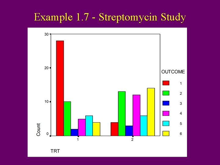
Side-by-Side Bar Charts • After Importing your dataset, and providing names to variables, click on: • GRAPHS BAR… Clustered (Summaries for Groups of Cases) DEFINE • Bars Represent N of Cases (or % of Cases) • CATEGORY AXIS: Variable that represents groups to be compared (independent variable) • DEFINE CLUSTERS BY: Variable that represents outcomes of interest (dependent variable)

Example 1. 7 - Streptomycin Study

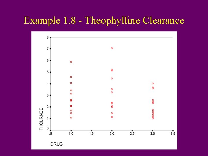
Scatterplots • After Importing your dataset, and providing names to variables, click on: • GRAPHS SCATTER SIMPLE DEFINE • For Y-AXIS, choose the Dependent (Response) Variable • For X-AXIS, choose the Independent (Explanatory) Variable

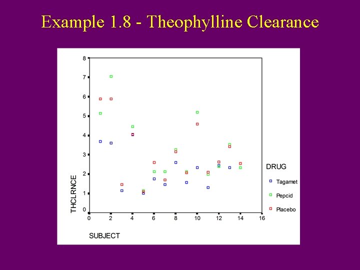
Example 1. 8 - Theophylline Clearance

Scatterplots with 2 Independent Variables • After Importing your dataset, and providing names to variables, click on: • GRAPHS SCATTER SIMPLE DEFINE • For Y-AXIS, choose the Dependent Variable • For X-AXIS, choose the Independent Variable with the most levels • For SET MARKERS BY, choose the Independent Variable with the fewest levels

Example 1. 8 - Theophylline Clearance

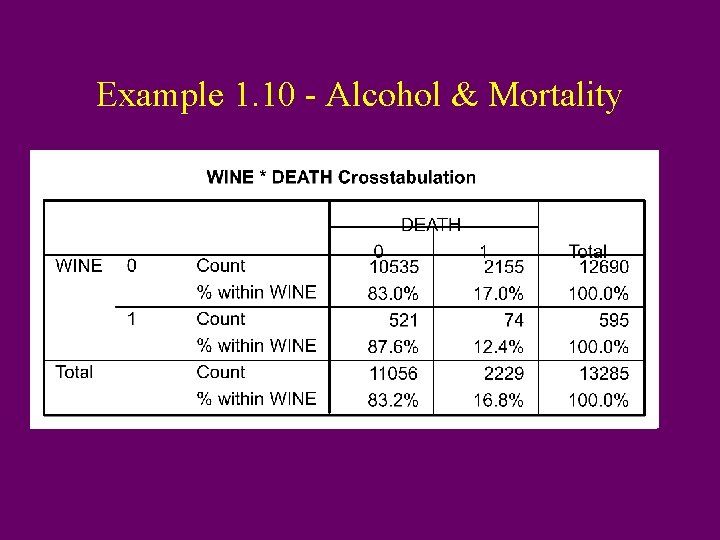
Contingency Tables for Conditional Probabilities • After Importing your dataset, and providing names to variables, click on: • ANALYZE DESCRIPTIVE STATISTICS CROSSTABS • For ROWS, select the variable you are conditioning on (Independent Variable) • For COLUMNS, select the variable you are finding the conditional probability of (Dependent Variable) • Click on CELLS • Click on ROW Percentages

Example 1. 10 - Alcohol & Mortality

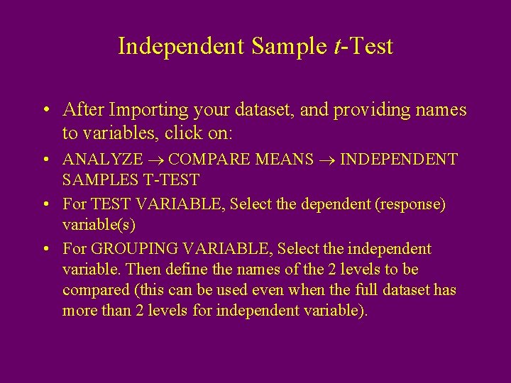
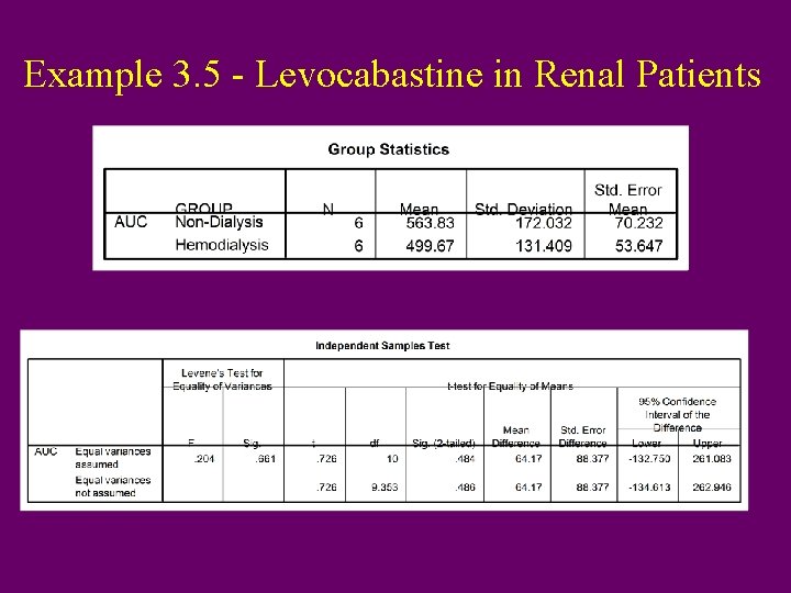
Independent Sample t-Test • After Importing your dataset, and providing names to variables, click on: • ANALYZE COMPARE MEANS INDEPENDENT SAMPLES T-TEST • For TEST VARIABLE, Select the dependent (response) variable(s) • For GROUPING VARIABLE, Select the independent variable. Then define the names of the 2 levels to be compared (this can be used even when the full dataset has more than 2 levels for independent variable).

Example 3. 5 - Levocabastine in Renal Patients

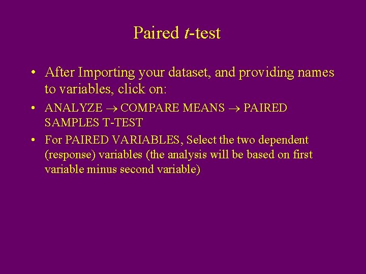
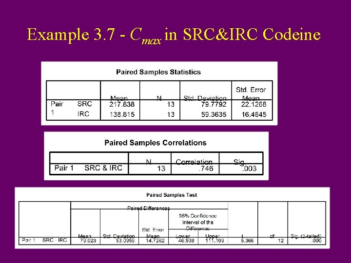
Paired t-test • After Importing your dataset, and providing names to variables, click on: • ANALYZE COMPARE MEANS PAIRED SAMPLES T-TEST • For PAIRED VARIABLES, Select the two dependent (response) variables (the analysis will be based on first variable minus second variable)

Example 3. 7 - Cmax in SRC&IRC Codeine

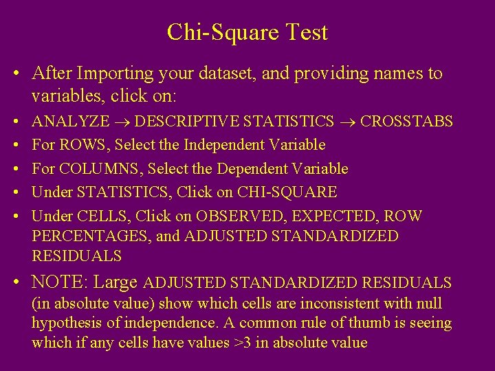
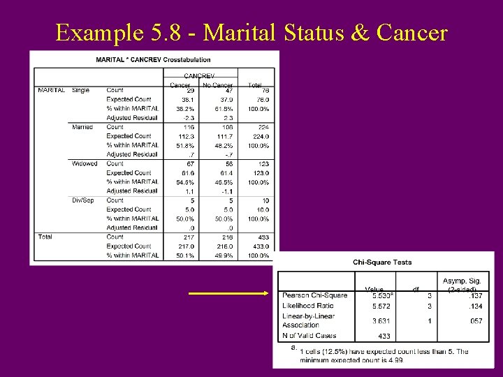
Chi-Square Test • After Importing your dataset, and providing names to variables, click on: • • • ANALYZE DESCRIPTIVE STATISTICS CROSSTABS For ROWS, Select the Independent Variable For COLUMNS, Select the Dependent Variable Under STATISTICS, Click on CHI-SQUARE Under CELLS, Click on OBSERVED, EXPECTED, ROW PERCENTAGES, and ADJUSTED STANDARDIZED RESIDUALS • NOTE: Large ADJUSTED STANDARDIZED RESIDUALS (in absolute value) show which cells are inconsistent with null hypothesis of independence. A common rule of thumb is seeing which if any cells have values >3 in absolute value

Example 5. 8 - Marital Status & Cancer

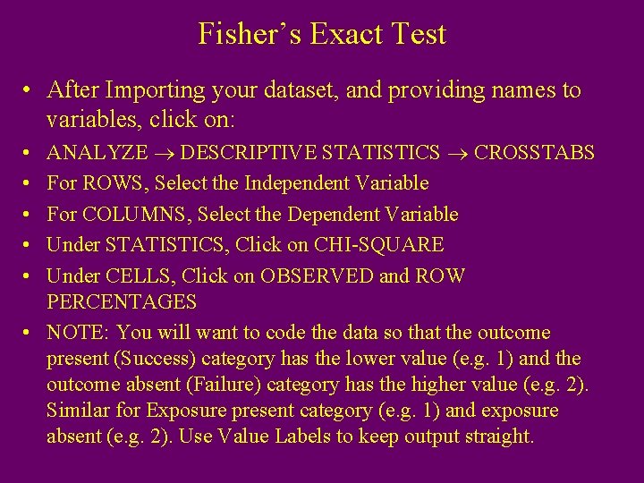
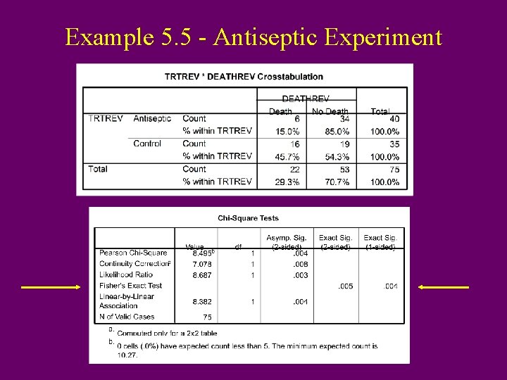
Fisher’s Exact Test • After Importing your dataset, and providing names to variables, click on: ANALYZE DESCRIPTIVE STATISTICS CROSSTABS For ROWS, Select the Independent Variable For COLUMNS, Select the Dependent Variable Under STATISTICS, Click on CHI-SQUARE Under CELLS, Click on OBSERVED and ROW PERCENTAGES • NOTE: You will want to code the data so that the outcome present (Success) category has the lower value (e. g. 1) and the outcome absent (Failure) category has the higher value (e. g. 2). Similar for Exposure present category (e. g. 1) and exposure absent (e. g. 2). Use Value Labels to keep output straight. • • •

Example 5. 5 - Antiseptic Experiment

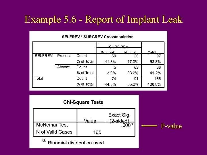
Mc. Nemar’s Test • After Importing your dataset, and providing names to variables, click on: ANALYZE DESCRIPTIVE STATISTICS CROSSTABS For ROWS, Select the outcome for condition/time 1 For COLUMNS, Select the outcome for condition/time 2 Under STATISTICS, Click on MCNEMAR Under CELLS, Click on OBSERVED and TOTAL PERCENTAGES • NOTE: You will want to code the data so that the outcome present (Success) category has the lower value (e. g. 1) and the outcome absent (Failure) category has the higher value (e. g. 2). Similar for Exposure present category (e. g. 1) and exposure absent (e. g. 2). Use Value Labels to keep output straight. • • •

Example 5. 6 - Report of Implant Leak P-value

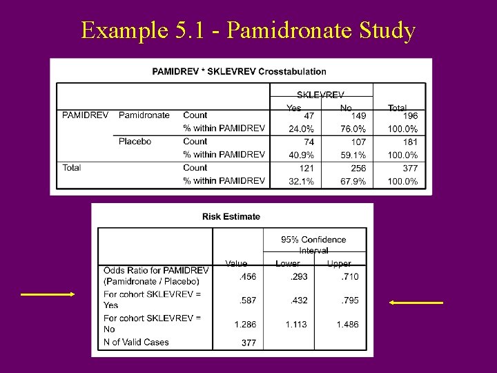
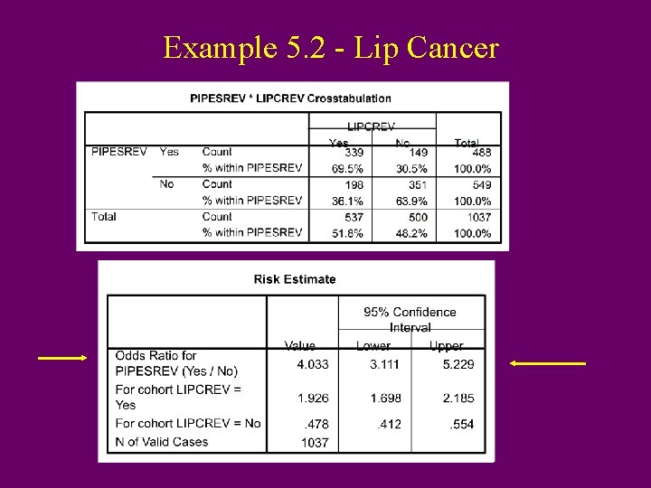
Relative Risks and Odds Ratios • After Importing your dataset, and providing names to variables, click on: • • • ANALYZE DESCRIPTIVE STATISTICS CROSSTABS For ROWS, Select the Independent Variable For COLUMNS, Select the Dependent Variable Under STATISTICS, Click on RISK Under CELLS, Click on OBSERVED and ROW PERCENTAGES NOTE: You will want to code the data so that the outcome present (Success) category has the lower value (e. g. 1) and the outcome absent (Failure) category has the higher value (e. g. 2). Similar for Exposure present category (e. g. 1) and exposure absent (e. g. 2). Use Value Labels to keep output straight.

Example 5. 1 - Pamidronate Study

Example 5. 2 - Lip Cancer

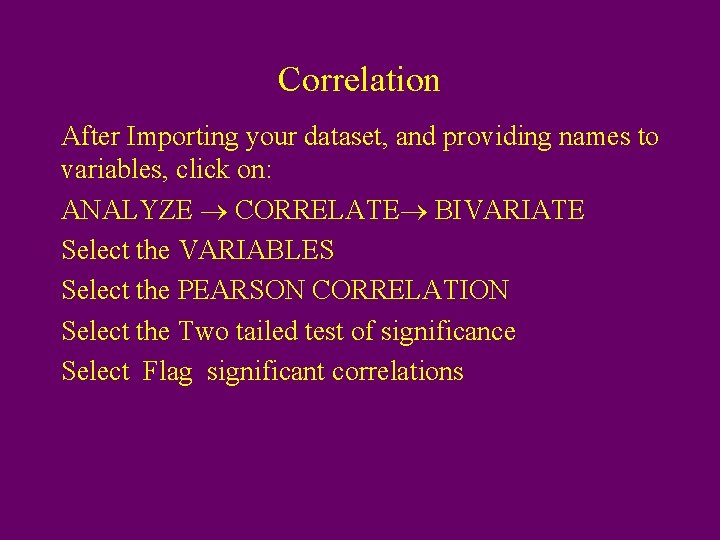
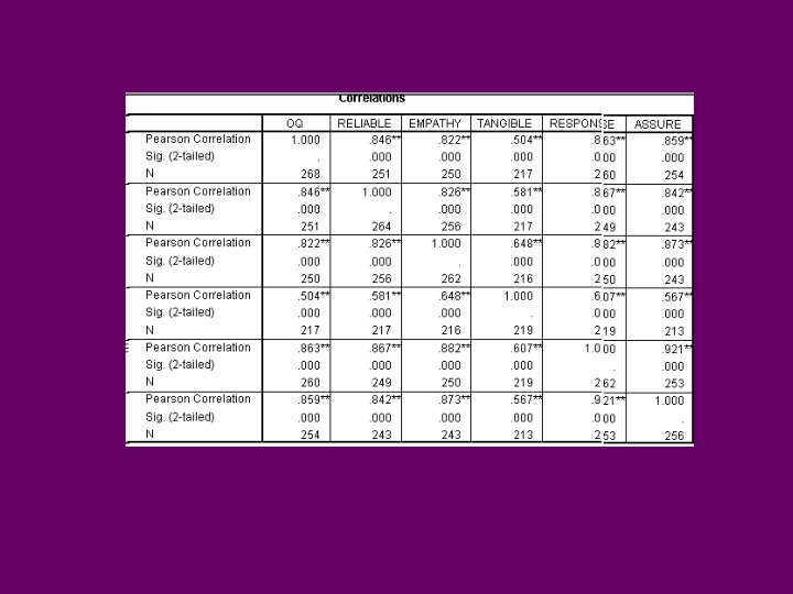
Correlation After Importing your dataset, and providing names to variables, click on: ANALYZE CORRELATE BIVARIATE Select the VARIABLES Select the PEARSON CORRELATION Select the Two tailed test of significance Select Flag significant correlations

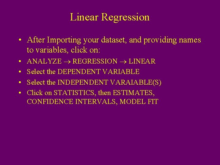
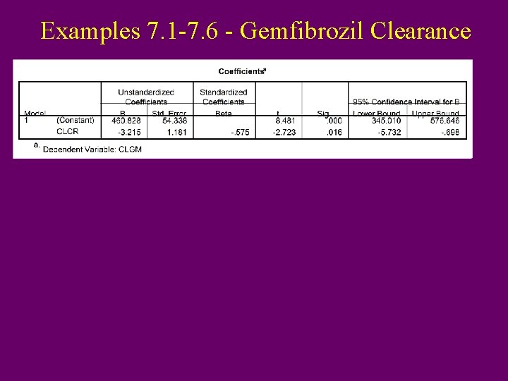
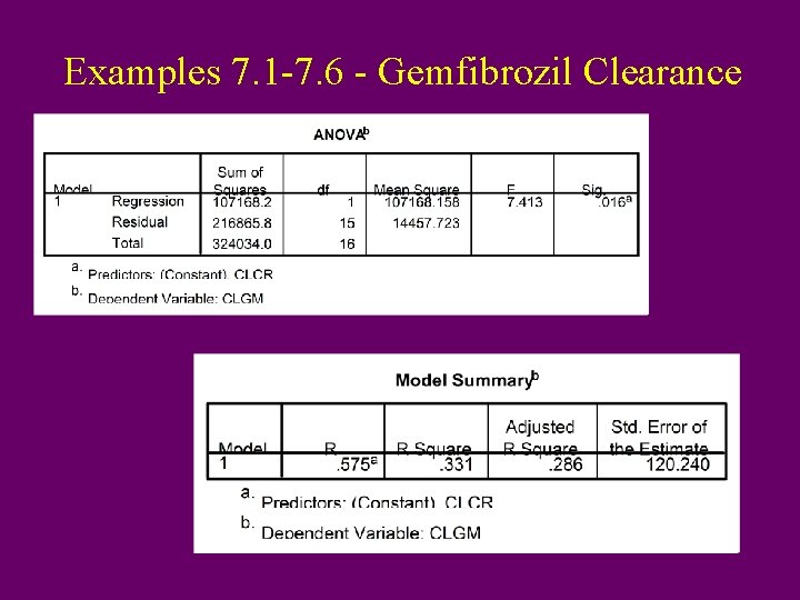
Linear Regression • After Importing your dataset, and providing names to variables, click on: • • ANALYZE REGRESSION LINEAR Select the DEPENDENT VARIABLE Select the INDEPENDENT VARAIABLE(S) Click on STATISTICS, then ESTIMATES, CONFIDENCE INTERVALS, MODEL FIT

Examples 7. 1 -7. 6 - Gemfibrozil Clearance

Examples 7. 1 -7. 6 - Gemfibrozil Clearance