Statistical Analysis of the Regression Discontinuity Design Analysis

Statistical Analysis of the Regression -Discontinuity Design

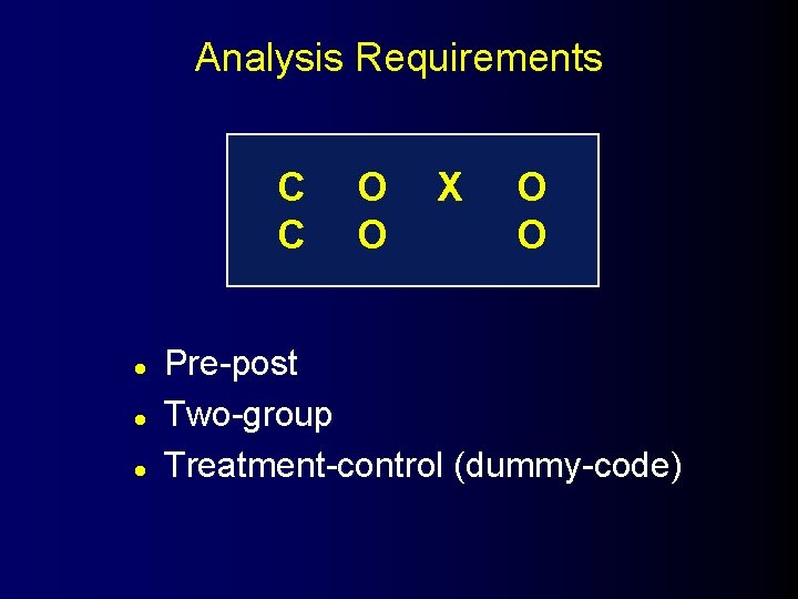
Analysis Requirements C C l l l O O X O O Pre-post Two-group Treatment-control (dummy-code)

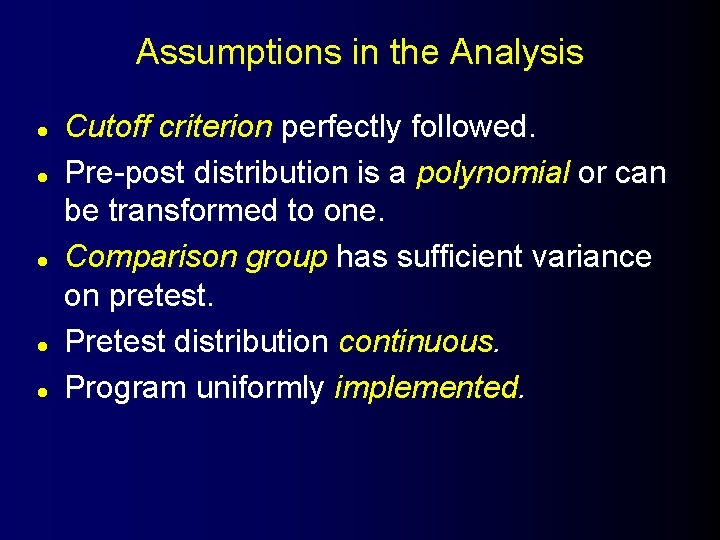
Assumptions in the Analysis l l l Cutoff criterion perfectly followed. Pre-post distribution is a polynomial or can be transformed to one. Comparison group has sufficient variance on pretest. Pretest distribution continuous. Program uniformly implemented.

The Curvilinearilty Problem If the true pre-post relationship is not linear. . . 80 posteff 70 60 50 40 30 20 0 10 20 30 40 50 pre 60 70 80 90 100

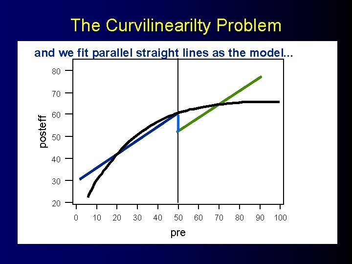
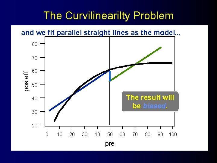
The Curvilinearilty Problem and we fit parallel straight lines as the model. . . 80 posteff 70 60 50 40 30 20 0 10 20 30 40 50 pre 60 70 80 90 100

The Curvilinearilty Problem and we fit parallel straight lines as the model. . . 80 posteff 70 60 50 The result will be biased. 40 30 20 0 10 20 30 40 50 pre 60 70 80 90 100

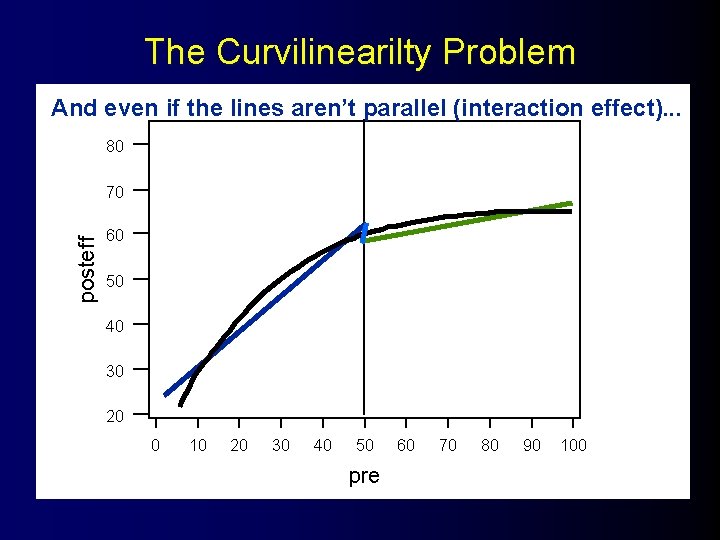
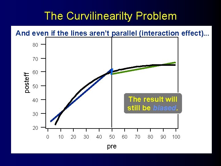
The Curvilinearilty Problem And even if the lines aren’t parallel (interaction effect). . . 80 posteff 70 60 50 40 30 20 0 10 20 30 40 50 pre 60 70 80 90 100

The Curvilinearilty Problem And even if the lines aren’t parallel (interaction effect). . . 80 posteff 70 60 50 The result will still be biased. 40 30 20 0 10 20 30 40 50 pre 60 70 80 90 100

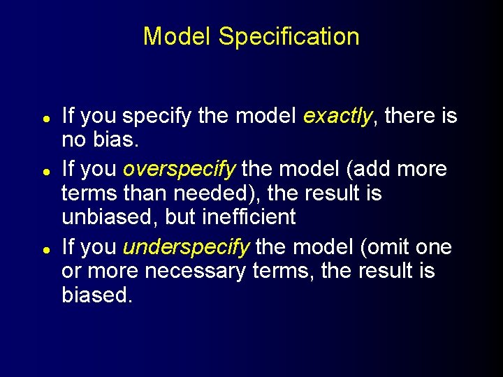
Model Specification l l l If you specify the model exactly, there is no bias. If you overspecify the model (add more terms than needed), the result is unbiased, but inefficient If you underspecify the model (omit one or more necessary terms, the result is biased.

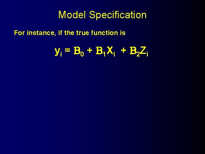
Model Specification For instance, if the true function is y i = 0 + 1 X i + 2 Z i

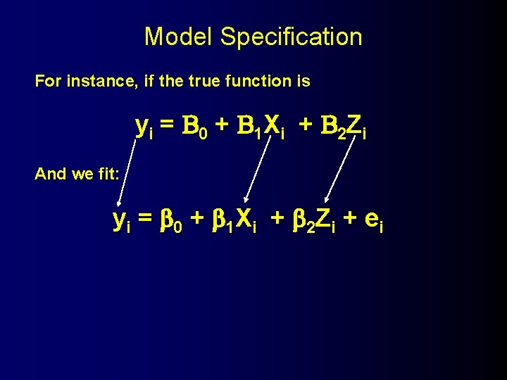
Model Specification For instance, if the true function is y i = 0 + 1 X i + 2 Z i And we fit: y i = 0 + 1 X i + 2 Z i + e i

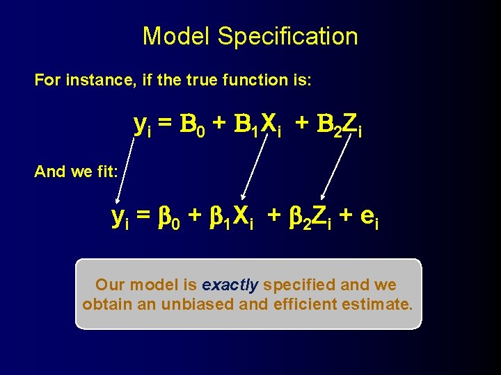
Model Specification For instance, if the true function is: y i = 0 + 1 X i + 2 Z i And we fit: y i = 0 + 1 X i + 2 Z i + e i Our model is exactly specified and we obtain an unbiased and efficient estimate.

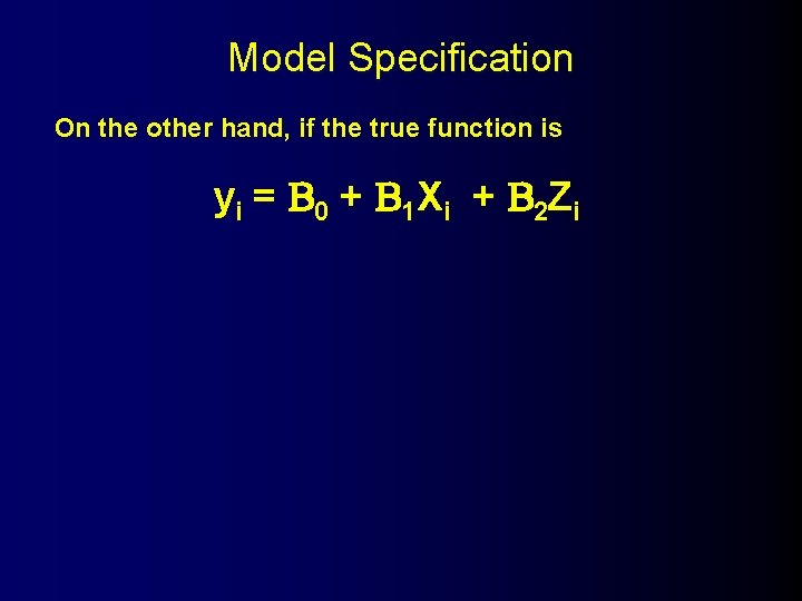
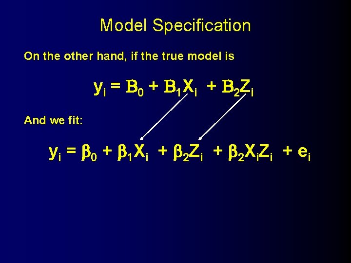
Model Specification On the other hand, if the true function is y i = 0 + 1 X i + 2 Z i

Model Specification On the other hand, if the true model is y i = 0 + 1 X i + 2 Z i And we fit: y i = 0 + 1 X i + 2 Z i + 2 X i Z i + e i

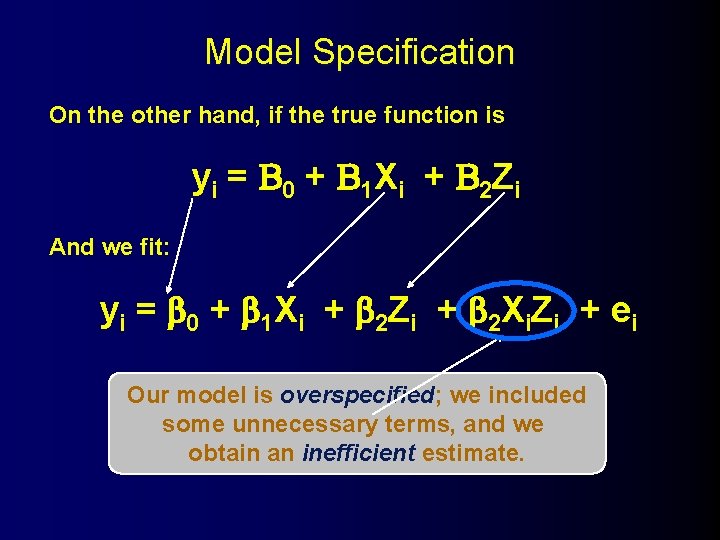
Model Specification On the other hand, if the true function is y i = 0 + 1 X i + 2 Z i And we fit: y i = 0 + 1 X i + 2 Z i + 2 X i Z i + e i Our model is overspecified; we included some unnecessary terms, and we obtain an inefficient estimate.

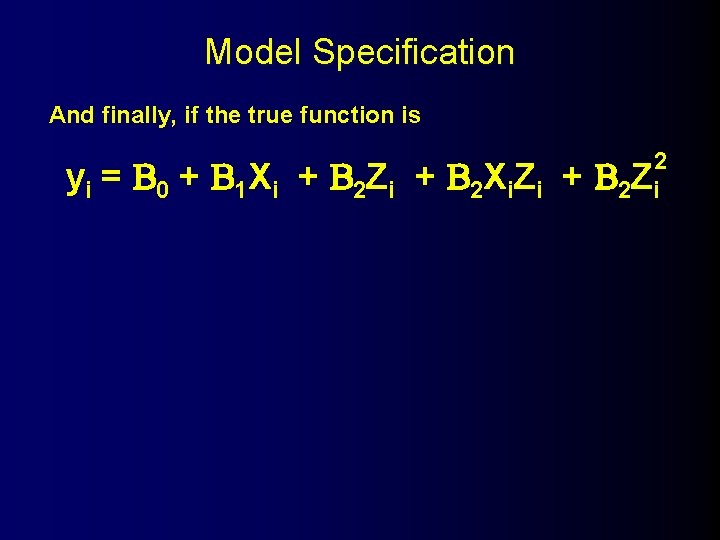
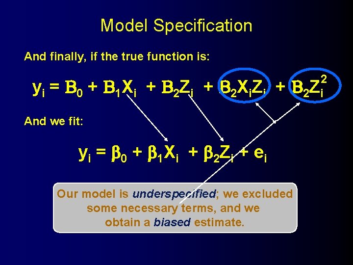
Model Specification And finally, if the true function is y i = 0 + 1 X i + 2 Z i + 2 X i Z i + 2 2 Z i

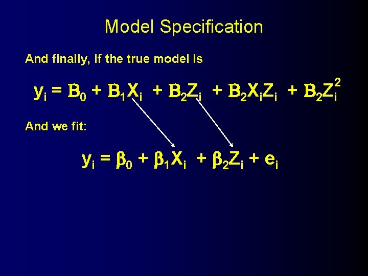
Model Specification And finally, if the true model is y i = 0 + 1 X i + 2 Z i + 2 X i Z i + And we fit: y i = 0 + 1 X i + 2 Z i + e i 2 2 Z i

Model Specification And finally, if the true function is: y i = 0 + 1 X i + 2 Z i + 2 X i Z i + 2 2 Z i And we fit: y i = 0 + 1 X i + 2 Z i + e i Our model is underspecified; we excluded some necessary terms, and we obtain a biased estimate.

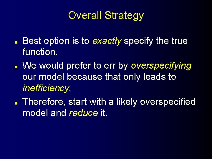
Overall Strategy l l l Best option is to exactly specify the true function. We would prefer to err by overspecifying our model because that only leads to inefficiency. Therefore, start with a likely overspecified model and reduce it.

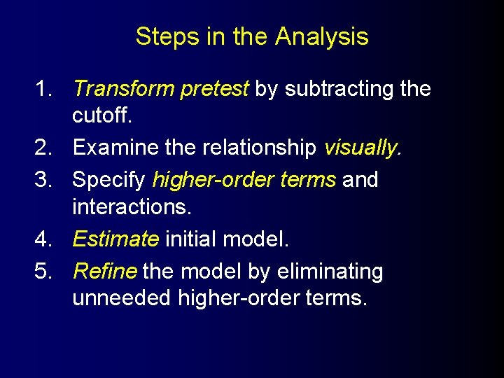
Steps in the Analysis 1. Transform pretest by subtracting the cutoff. 2. Examine the relationship visually. 3. Specify higher-order terms and interactions. 4. Estimate initial model. 5. Refine the model by eliminating unneeded higher-order terms.

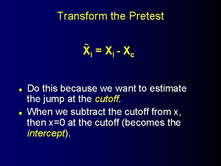
Transform the Pretest ~ Xi = X i - X c l l Do this because we want to estimate the jump at the cutoff. When we subtract the cutoff from x, then x=0 at the cutoff (becomes the intercept).

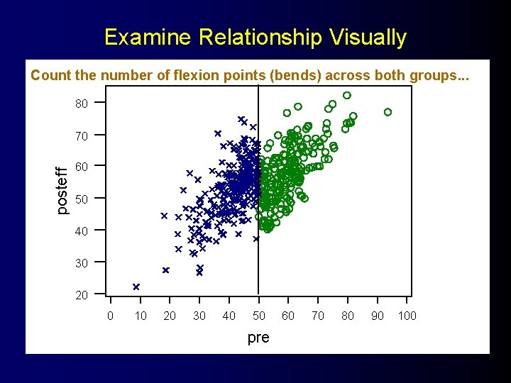
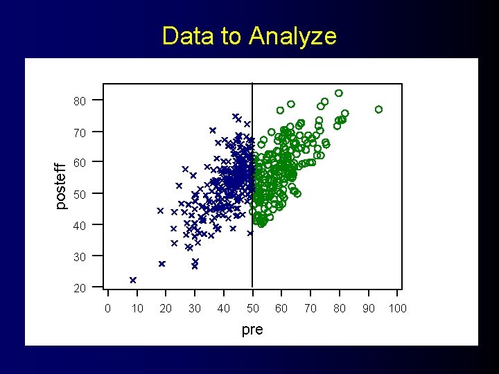
Examine Relationship Visually Count the number of flexion points (bends) across both groups. . . 80 posteff 70 60 50 40 30 20 0 10 20 30 40 50 pre 60 70 80 90 100

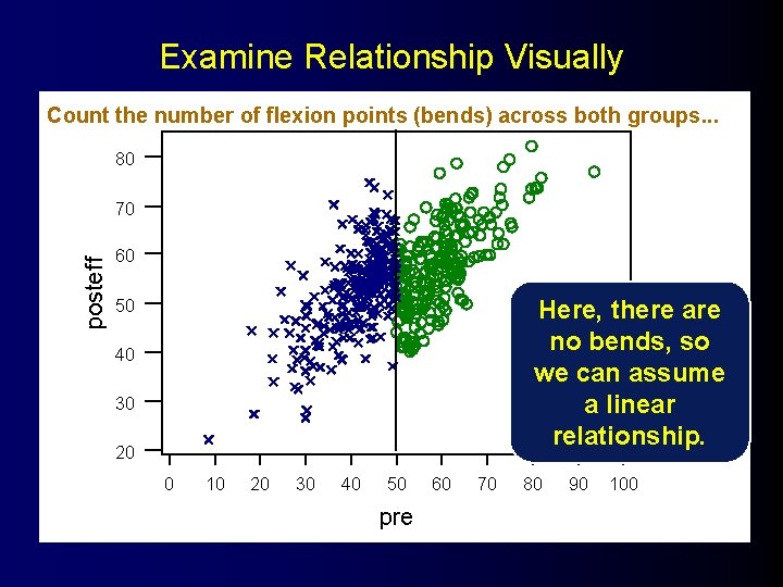
Examine Relationship Visually Count the number of flexion points (bends) across both groups. . . 80 posteff 70 60 50 Here, there are no bends, so we can assume a linear relationship. 40 30 20 0 10 20 30 40 50 pre 60 70 80 90 100

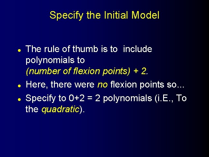
Specify the Initial Model l The rule of thumb is to include polynomials to (number of flexion points) + 2. Here, there were no flexion points so. . . Specify to 0+2 = 2 polynomials (i. E. , To the quadratic).

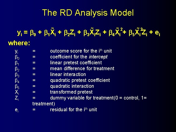
The RD Analysis Model ~ ~ y i = 0 + 1 X i + 2 Z i + 3 X i Z i + ~2 4 X i + ~2 5 X i Z i where: yi 0 1 2 3 4 5 Xi Zi ei = outcome score for the ith unit = coefficient for the intercept = linear pretest coefficient = mean difference for treatment = linear interaction = quadratic pretest coefficient = quadratic interaction = transformed pretest = dummy variable for treatment(0 = control, 1= treatment) = residual for the ith unit + ei

Data to Analyze 80 posteff 70 60 50 40 30 20 0 10 20 30 40 50 pre 60 70 80 90 100

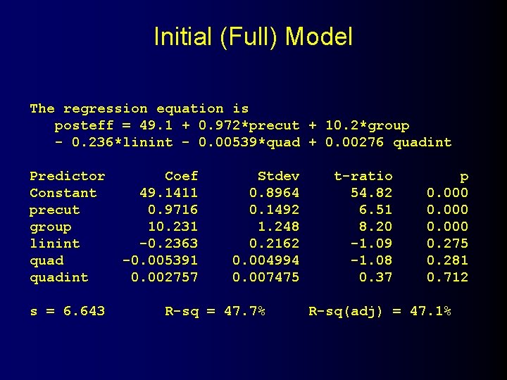
Initial (Full) Model The regression equation is posteff = 49. 1 + 0. 972*precut + 10. 2*group - 0. 236*linint - 0. 00539*quad + 0. 00276 quadint Predictor Constant precut group linint quadint s = 6. 643 Coef 49. 1411 0. 9716 10. 231 -0. 2363 -0. 005391 0. 002757 Stdev 0. 8964 0. 1492 1. 248 0. 2162 0. 004994 0. 007475 R-sq = 47. 7% t-ratio 54. 82 6. 51 8. 20 -1. 09 -1. 08 0. 37 p 0. 000 0. 275 0. 281 0. 712 R-sq(adj) = 47. 1%

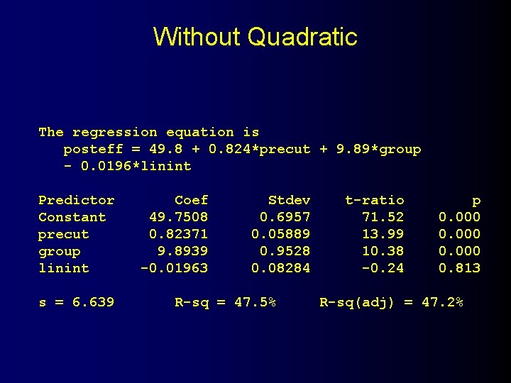
Without Quadratic The regression equation is posteff = 49. 8 + 0. 824*precut + 9. 89*group - 0. 0196*linint Predictor Constant precut group linint s = 6. 639 Coef 49. 7508 0. 82371 9. 8939 -0. 01963 Stdev 0. 6957 0. 05889 0. 9528 0. 08284 R-sq = 47. 5% t-ratio 71. 52 13. 99 10. 38 -0. 24 p 0. 000 0. 813 R-sq(adj) = 47. 2%

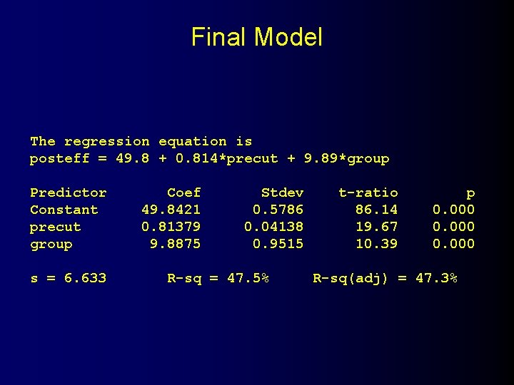
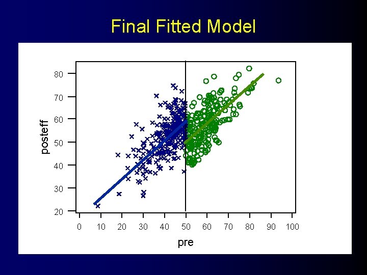
Final Model The regression equation is posteff = 49. 8 + 0. 814*precut + 9. 89*group Predictor Constant precut group s = 6. 633 Coef 49. 8421 0. 81379 9. 8875 Stdev 0. 5786 0. 04138 0. 9515 R-sq = 47. 5% t-ratio 86. 14 19. 67 10. 39 p 0. 000 R-sq(adj) = 47. 3%

Final Fitted Model 80 posteff 70 60 50 40 30 20 0 10 20 30 40 50 pre 60 70 80 90 100