Statistical Analysis of Longitudinal Data Ziad Taib Biostatistics

Statistical Analysis of Longitudinal Data Ziad Taib Biostatistics, AZ April 2011 Name, department 1 Date

Outline of lecture 1 1. An introduction 2. Two examples 3. Principles of Inference 4. Modelling continuous longitudinal data Name, department 2 Date

Part 1: An introduction Name, department 3 Date

Why longitudinal data? § Very useful for their own sake. § With longitudinal data, we have the possibility of understanding what mixed models are about in a relatively simple but yet rich enough context. __________________ A good reference is the book ”Designing experiments and analyzing data” by Maxwel l& Delaney (2004) Name, department 4 Date

Longitudinal Data Repeated measures are obtained when a response is measured repeatedly on a set of units • Units: • Subjects, patients, participants, . . . • indivduals, plants, . . . • Clusters: nests, families, towns, . . • Special case: Longitudinal data Obs! Possible to handle several levels Name, department 5 Date

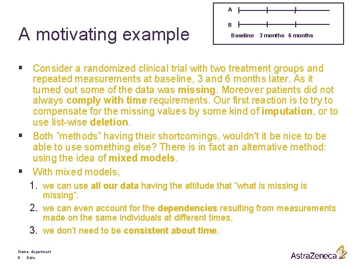
A A motivating example B Baseline 3 months 6 months § Consider a randomized clinical trial with two treatment groups and repeated measurements at baseline, 3 and 6 months later. As it turned out some of the data was missing. Moreover patients did not always comply with time requirements. Our first reaction is to try to compensate for the missing values by some kind of imputation, or to use list-wise deletion. § Both ”methods” having their shortcomings, wouldn't it be nice to be able to use something else? There is in fact an alternative method: using the idea of mixed models. § With mixed models, 1. we can use all our data having the attitude that ”what is missing”. 2. we can even account for the dependencies resulting from measurements made on the same individuals at different times. 3. we don’t need to be consistent about time. Name, department 6 Date

Mixed effects models § Ordinary fixed effects linear model usually assume: 1) independence with the same variance. 2) normally distributed errors. 3) constant parameters § If we modify assumptions 1) and 3), then the problem becomes more complicated and in general we need a large number of parameters only to describe the covariance structure of the observations. Mixed effects models deal with this type of problems. § In general, this type of models allows us to tackle such problems as: clustered data, repeated measures, hierarchical data. Name, department 7 Date

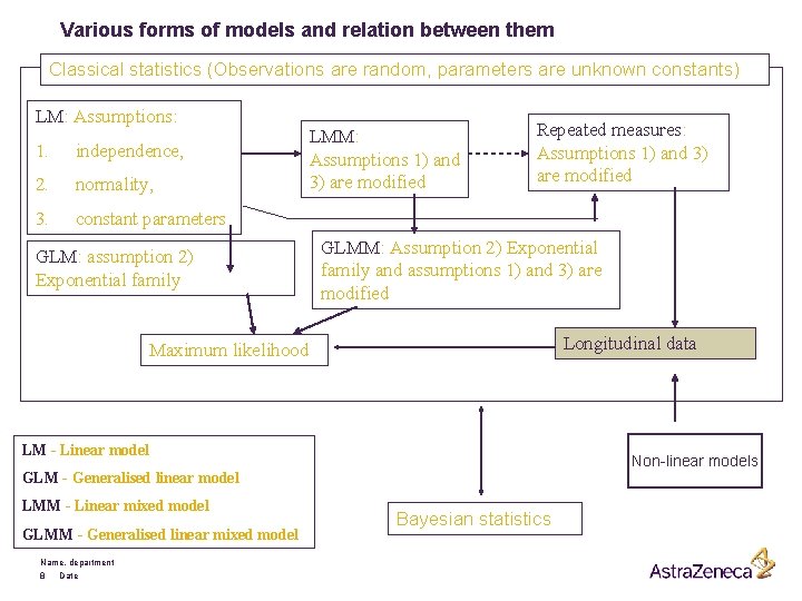
Various forms of models and relation between them Classical statistics (Observations are random, parameters are unknown constants) LM: Assumptions: 1. independence, 2. normality, 3. constant parameters GLM: assumption 2) Exponential family LMM: Assumptions 1) and 3) are modified Repeated measures: Assumptions 1) and 3) are modified GLMM: Assumption 2) Exponential family and assumptions 1) and 3) are modified Longitudinal data Maximum likelihood LM - Linear model Non-linear models GLM - Generalised linear model LMM - Linear mixed model GLMM - Generalised linear mixed model Name, department 8 Date Bayesian statistics

Part 2: Two examples § Rat data § Prostate data Name, department 9 Date

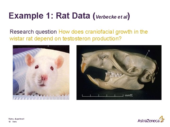
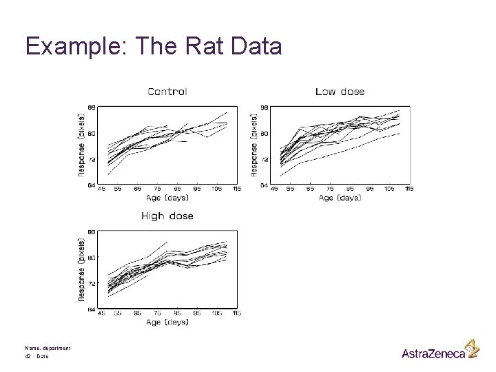
Example 1: Rat Data (Verbecke et al) Research question How does craniofacial growth in the wistar rat depend on testosteron production? Name, department 10 Date

e s n d e i ) f i e l t p ria m i S iva (un Name, department 11 Date po s re

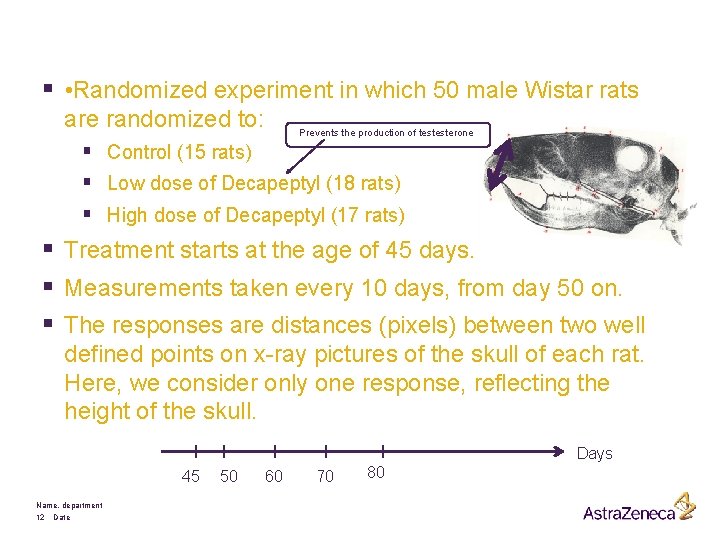
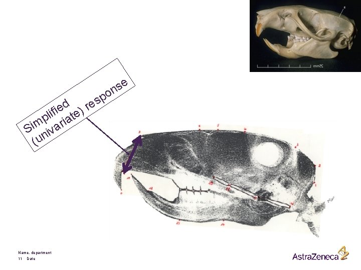
§ • Randomized experiment in which 50 male Wistar rats are randomized to: Prevents the production of testesterone § Control (15 rats) § Low dose of Decapeptyl (18 rats) § High dose of Decapeptyl (17 rats) § Treatment starts at the age of 45 days. § Measurements taken every 10 days, from day 50 on. § The responses are distances (pixels) between two well defined points on x-ray pictures of the skull of each rat. Here, we consider only one response, reflecting the height of the skull. Days 45 Name, department 12 Date 50 60 70 80

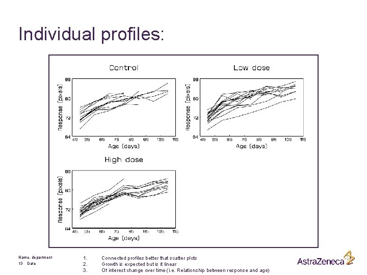
Individual profiles: Name, department 13 Date 1. 2. 3. Connected profiles better that scatter plots Growth is expected but is it linear Of interest change over time (i. e. Relationship between response and age)

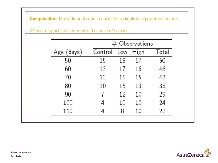
Complication: Many dropouts due to anaesthesia imply less power but no bias. Without dropouts easier problem because of balance. Name, department 14 Date

Remarks: § Much variability between rats § Much less variability within rats § Fixed number of measurements scheduled per subject, but not all measurements available due to dropout, for known reason. § Measurements taken at fixed time points Research question: How does craniofacial growth in the wistar rat depend on testosteron production ? Name, department 15 Date

Example 2: The BLSA Prostate Data Name, department 16 Date

Example 2: The BLSA Prostate Data (Pearson et al. , Statistics in Medicine, 1994). § Prostate disease is one of the most common and most costly medical problems in the world. Important to look for biomarkers which can detect the disease at an early stage. § Prostate-Specific Antigen is an enzyme produced by both normal and cancerous prostate cells. It is believed that PSA level is related to the volume of prostate tissue. § Problem: Patients with Benign Prostatic Hyperplasia also have an increased PSA level § Overlap in PSA distribution for cancer and BPH cases seriously complicates the detection of prostate cancer. Name, department 17 Date

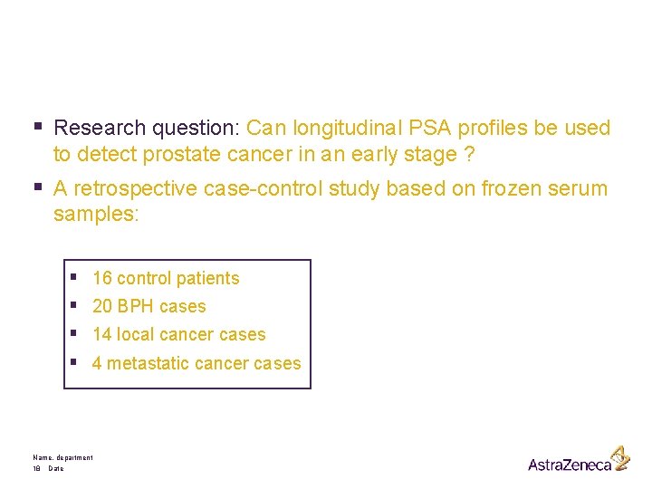
§ Research question: Can longitudinal PSA profiles be used to detect prostate cancer in an early stage ? § A retrospective case-control study based on frozen serum samples: § § 16 control patients 20 BPH cases 14 local cancer cases 4 metastatic cancer cases Name, department 18 Date

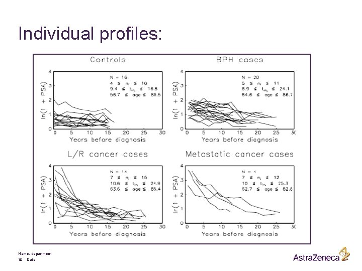
Individual profiles: Name, department 19 Date

Remarks: § Much variability between subjects § Little variability within subjects § Highly unbalanced data Research question: Can longitudinal PSA profiles be used to detect prostate cancer in an early stage ? Name, department 20 Date

Part 3: Principles of Inference Name, department 21 Date

Fisher´s likelihood Inference for observable y and fixed parameter q § Data Generation : Given a stochastic model , Generate data, y, from § Parameter Estimation : Given the data y, make inference about q by using the likelihood § Connection between two processes : Name, department 22 Date

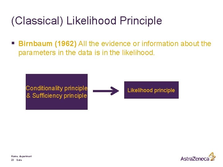
(Classical) Likelihood Principle § Birnbaum (1962) All the evidence or information about the parameters in the data is in the likelihood. Conditionality principle & Sufficiency principle Name, department 23 Date Likelihood principle

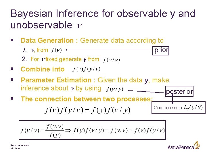
Bayesian Inference for observable y and unobservable n § Data Generation : Generate data according to 1. n, from prior 2. For n fixed generate y from § Combine into § Parameter Estimation : Given the data y, make inference about n by using § The connection between two processes: posterior Compare with Name, department 24 Date

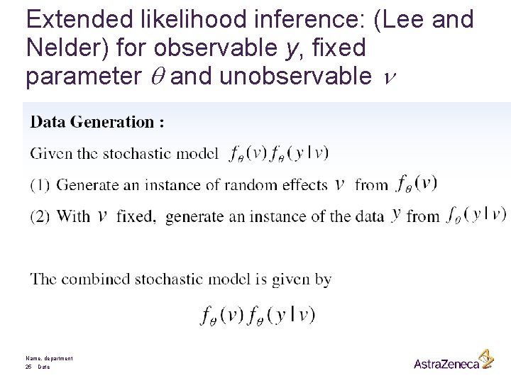
Extended likelihood inference: (Lee and Nelder) for observable y, fixed parameter q and unobservable n Name, department 25 Date

Parameter estimation Name, department 26 Date

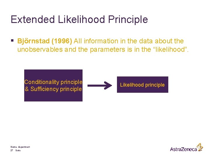
Extended Likelihood Principle § Björnstad (1996) All information in the data about the unobservables and the parameters is in the “likelihood”. Conditionality principle & Sufficiency principle Name, department 27 Date Likelihood principle

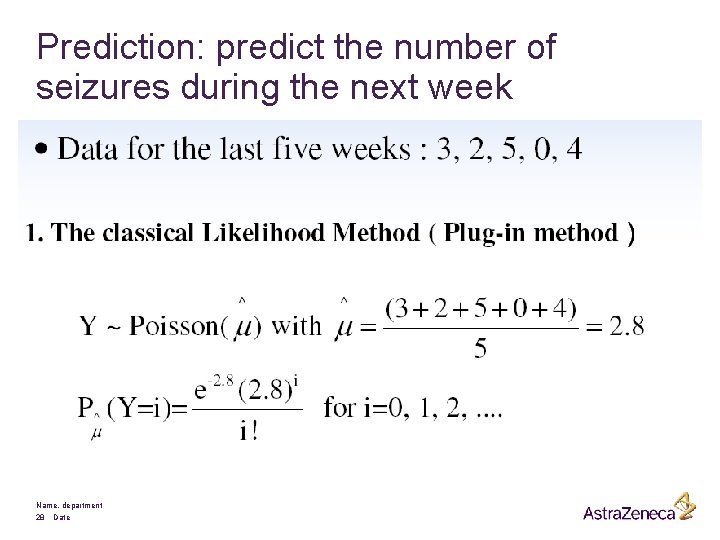
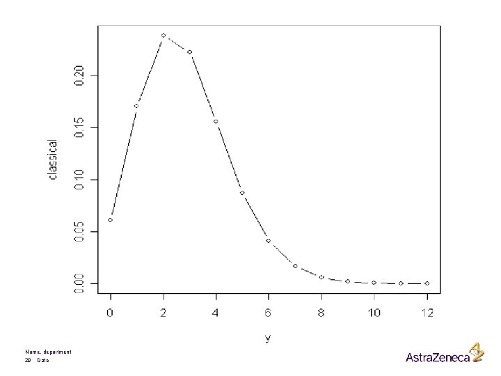
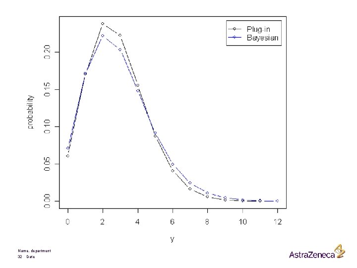
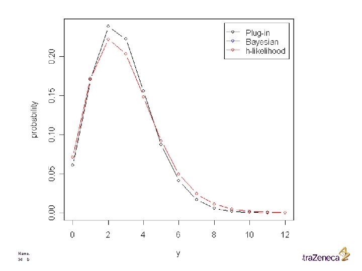
Prediction: predict the number of seizures during the next week Name, department 28 Date

Name, department 29 Date

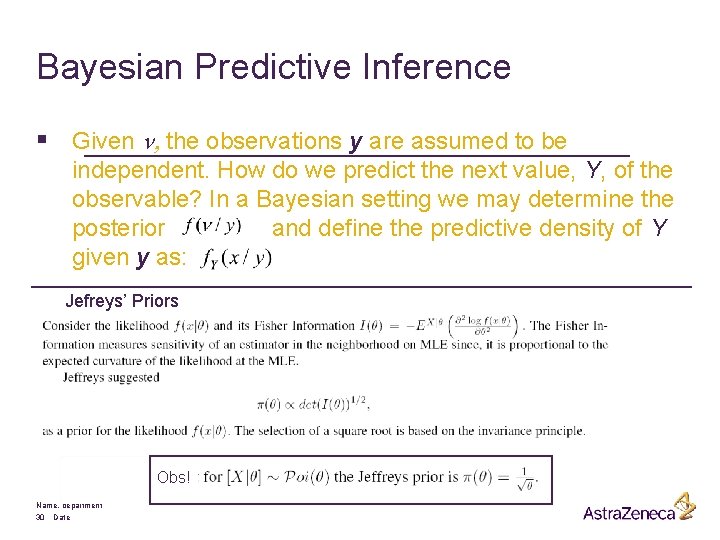
Bayesian Predictive Inference § Given n, the observations y are assumed to be independent. How do we predict the next value, Y, of the observable? In a Bayesian setting we may determine the posterior and define the predictive density of Y given y as: Jefreys’ Priors Obs! Name, department 30 Date

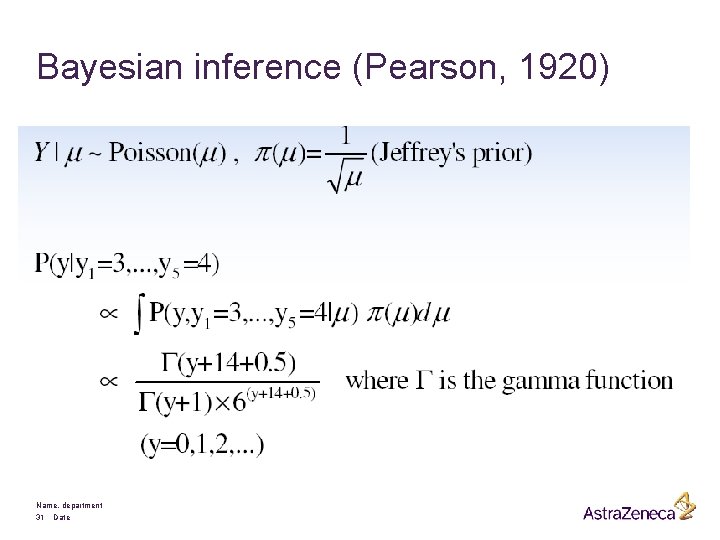
Bayesian inference (Pearson, 1920) Name, department 31 Date

Name, department 32 Date

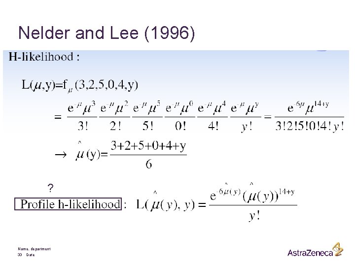
Nelder and Lee (1996) ? Name, department 33 Date

Name, department 34 Date

Part 4: A Model for Longitudinal Data Name, department 35 Date

Introduction § In practice: often unbalanced data due to § (i) unequal number of measurements per subject § (ii) measurements not taken at fixed time points. Therefore, ordinary multivariate regression techniques are often not applicable. § Often, subject-specific longitudinal profiles can be well approximated by linear regression functions. This leads to a 2 -stage model formulation: § Stage 1: A linear (e. g. regression) model for each subject separately § Stage 2: Explain variability in the subject-specific (regression) coefficients using known covariates Name, department 36 Date

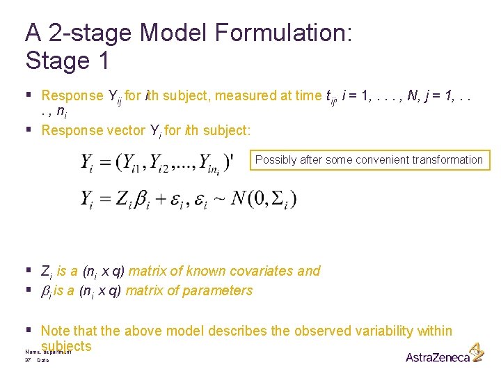
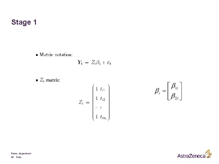
A 2 -stage Model Formulation: Stage 1 § Response Yij for ith subject, measured at time tij, i = 1, . . . , N, j = 1, . . . , ni § Response vector Yi for ith subject: Possibly after some convenient transformation § Zi is a (ni x q) matrix of known covariates and § bi is a (ni x q) matrix of parameters § Note that the above model describes the observed variability within subjects Name, department 37 Date

Stage 2 § Between-subject variability can now be studied from relating the parameters bi to known covariates § Ki is a (q x p) matrix of known covariates and § b is a (p-dimensional vector of unknown regression parameters § Finally Name, department 38 Date

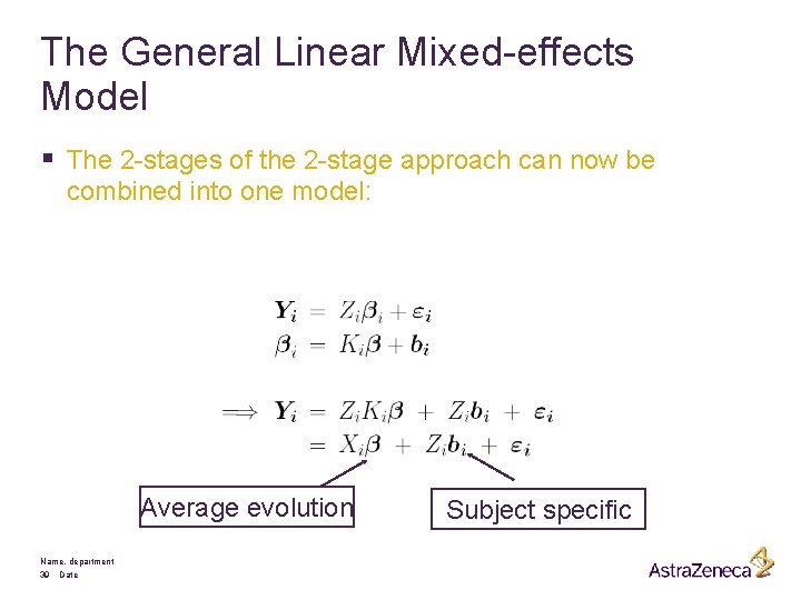
The General Linear Mixed-effects Model § The 2 -stages of the 2 -stage approach can now be combined into one model: Average evolution Name, department 39 Date Subject specific

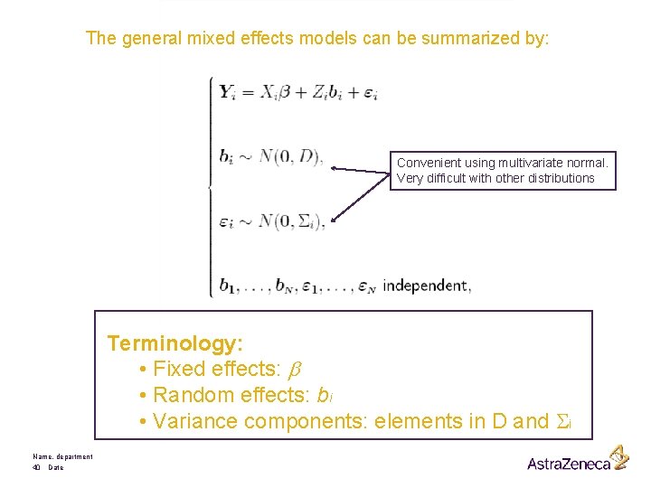
The general mixed effects models can be summarized by: Convenient using multivariate normal. Very difficult with other distributions Terminology: • Fixed effects: b • Random effects: bi • Variance components: elements in D and Si Name, department 40 Date

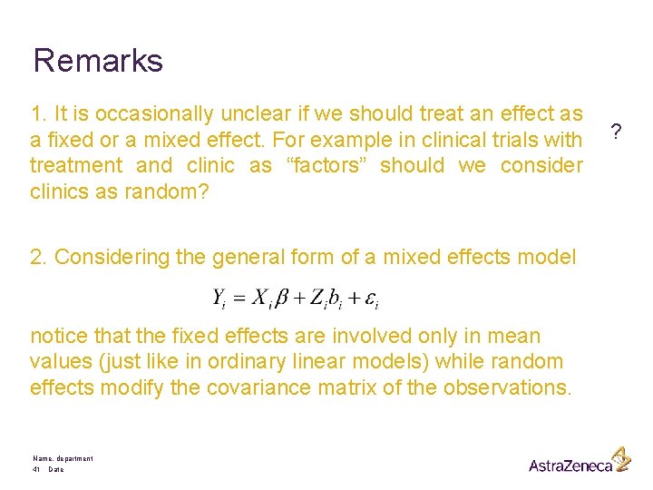
Remarks 1. It is occasionally unclear if we should treat an effect as a fixed or a mixed effect. For example in clinical trials with treatment and clinic as “factors” should we consider clinics as random? 2. Considering the general form of a mixed effects model notice that the fixed effects are involved only in mean values (just like in ordinary linear models) while random effects modify the covariance matrix of the observations. Name, department 41 Date ?

Example: The Rat Data Name, department 42 Date

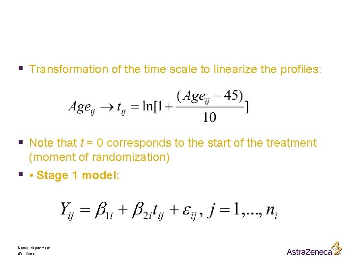
§ Transformation of the time scale to linearize the profiles: § Note that t = 0 corresponds to the start of the treatment (moment of randomization) § • Stage 1 model: Name, department 43 Date

Stage 1 Name, department 44 Date

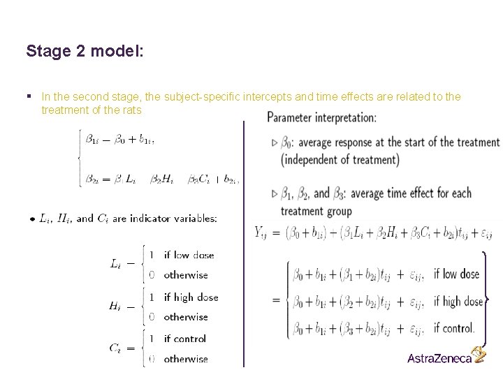
Stage 2 model: § In the second stage, the subject-specific intercepts and time effects are related to the treatment of the rats Name, department 45 Date

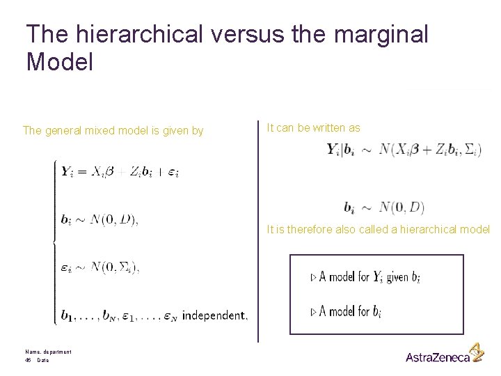
The hierarchical versus the marginal Model The general mixed model is given by It can be written as It is therefore also called a hierarchical model Name, department 46 Date

Marginally we have that is distributed as Hence Name, department 47 Date f(yi I bi) f(yi)

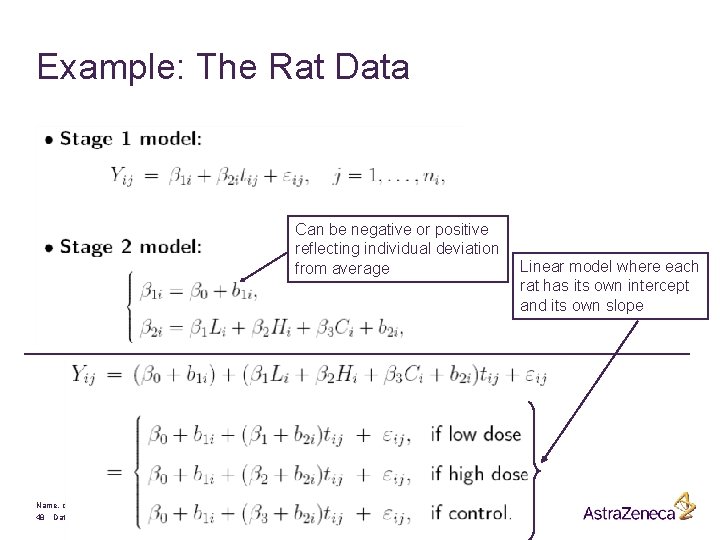
Example: The Rat Data Can be negative or positive reflecting individual deviation from average Name, department 48 Date Linear model where each rat has its own intercept and its own slope

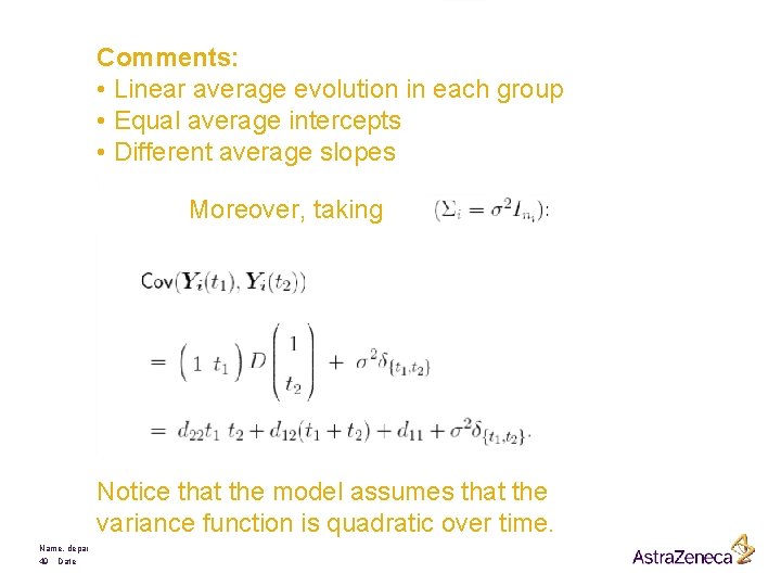
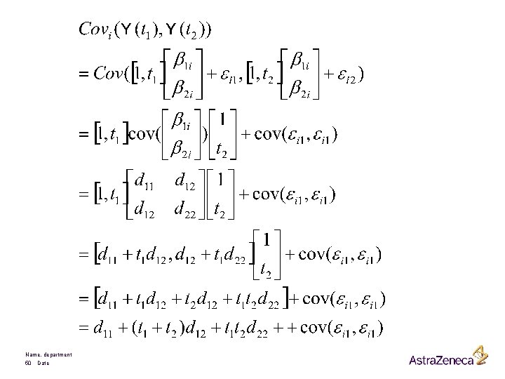
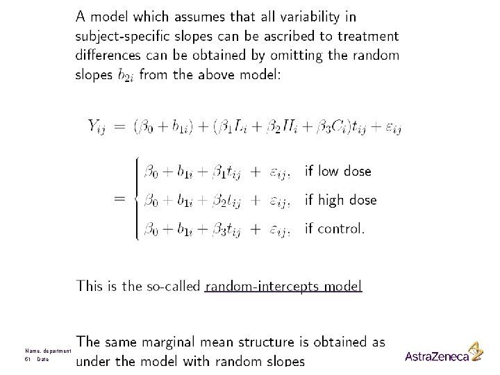
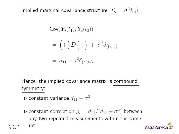
Comments: • Linear average evolution in each group • Equal average intercepts • Different average slopes Moreover, taking Notice that the model assumes that the variance function is quadratic over time. Name, department 49 Date

Name, department 50 Date

Name, department 51 Date

Name, department 52 Date

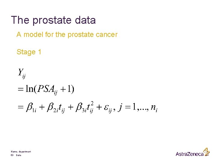
The prostate data A model for the prostate cancer Stage 1 Name, department 53 Date

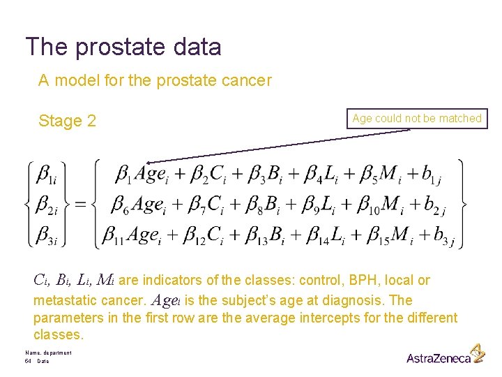
The prostate data A model for the prostate cancer Stage 2 Age could not be matched Ci, Bi, Li, Mi are indicators of the classes: control, BPH, local or metastatic cancer. Agei is the subject’s age at diagnosis. The parameters in the first row are the average intercepts for the different classes. Name, department 54 Date

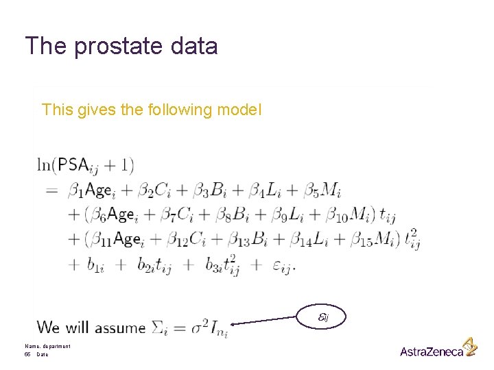
The prostate data This gives the following model eij Name, department 55 Date

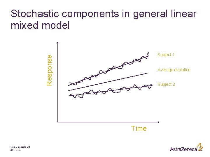
Stochastic components in general linear mixed model Response Subject 1 Average evolution Subject 2 Time Name, department 56 Date

References § Aerts, M. , Geys, H. , Molenberghs, G. , and Ryan, L. M. (2002). Topics in Modelling of Clustered Data. London: Chapman and Hall. § • Brown, H. and Prescott, R. (1999). Applied Mixed Models in Medicine. New-York: John Wiley & Sons. § • Crowder, M. J. and Hand, D. J. (1990). Analysis of Repeated Measures. London: Chapman and Hall. § • Davidian, M. and Giltinan, D. M. (1995). Nonlinear Models For Repeated Measurement Data. London: Chapman and Hall. § Davis, C. S. (2002). Statistical Methods for the Analysis of Repeated Measurements. New York: Springer-Verlag. § Diggle, P. J. , Heagerty, P. J. , Liang, K. Y. and Zeger, S. L. (2002). Analysis of Longitudinal Data. (2 nd edition). Oxford: Oxford University Press. Name, department 57 Date

References § Fahrmeir, L. and Tutz, G. (2002). Multivariate Statistical Modelling § § § § Based on Generalized Linear Models, (2 nd edition). Springer Series in Statistics. New-York: Springer-Verlag. Goldstein, H. (1979). The Design and Analysis of Longitudinal Studies. London: Academic Press. Goldstein, H. (1995). Multilevel Statistical Models. London: Edward Arnold. Hand, D. J. and Crowder, M. J. (1995). Practical Longitudinal Data Analysis. London: Chapman and Hall. Jones, B. and Kenward, M. G. (1989). Design and Analysis of Crossover Trials. London: Chapman and Hall. Kshirsagar, A. M. and Smith, W. B. (1995). Growth Curves. New-York: Marcel Dekker. Lindsey, J. K. (1993). Models for Repeated Measurements. Oxford: Oxford University Press. Longford, N. T. (1993). Random Coefficient Models. Oxford: Oxford University Press. Name, department 58 Date

References § Pinheiro, J. C. and Bates D. M. (2000). Mixed effects models in S and S -Plus, Springer Series in Statistics and Computing. New-York: Springer -Verlag. § Searle, S. R. , Casella, G. , and Mc. Culloch, C. E. (1992). Variance Components. New-York: Wiley. § Senn, S. J. (1993). Cross-over Trials in Clinical Research. Chichester: Wiley. § Verbeke, G. and Molenberghs, G. (1997). Linear Mixed Models In Practice: A SAS Oriented Approach, Lecture Notes in Statistics 126. New-York: Springer-Verlag. § Verbeke, G. and Molenberghs, G. (2000). Linear Mixed Models for Longitudinal Data. Springer Series in Statistics. New-York: Springer. Verlag. § Vonesh, E. F. and Chinchilli, V. M. (1997). Linear and Non-linear Models for the Analysis of Repeated Measurements. Marcel Dekker: Name, department 59 Date

Any Questions Name, department 60 Date ?