Statistical Analysis of Geographical Information Dr Marina Gavrilova

Statistical Analysis of Geographical Information Dr. Marina Gavrilova 1

Topics � Introduction � Distribution Descriptors: One Variable � Relationship Descriptors: Two Variables � Point Pattern Descriptors � Point Pattern Analyzers � Autocorrelation 2

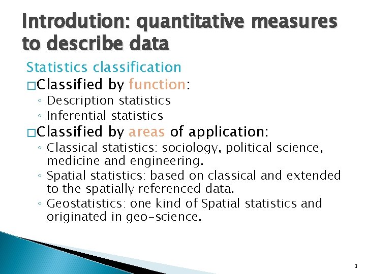
Introdution: quantitative measures to describe data Statistics classification � Classified by function: ◦ Description statistics ◦ Inferential statistics � Classified by areas of application: ◦ Classical statistics: sociology, political science, medicine and engineering. ◦ Spatial statistics: based on classical and extended to the spatially referenced data. ◦ Geostatistics: one kind of Spatial statistics and originated in geo-science. 3

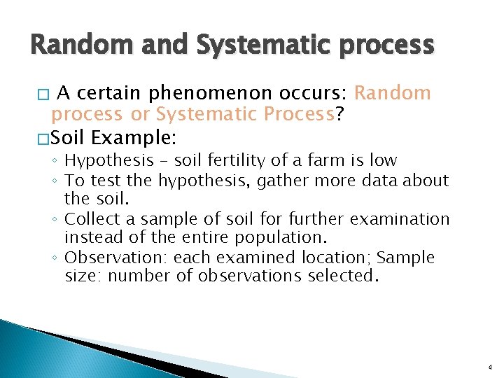
Random and Systematic process A certain phenomenon occurs: Random process or Systematic Process? � Soil Example: � ◦ Hypothesis – soil fertility of a farm is low ◦ To test the hypothesis, gather more data about the soil. ◦ Collect a sample of soil for further examination instead of the entire population. ◦ Observation: each examined location; Sample size: number of observations selected. 4

Features about spatial data(1) A region can be partitioned in many ways based on the given criteria. USA: States boundaries, census geography. Modifiable Area Unit Problem (MAUP) include: ◦ Scale effect: Analyze data at multiple levels of spatial resolution results in inconsistency. ◦ Zoning effect: Analyze data derived from different zonal systems with similar number of areal units results in inconsistency. 5

Features about spatial data(2) Spatial autocorrelation represents the nature of geography and, consequently, will almost always be present in spatial data. Tober “First Law of Geography”: “All things related to each other, but closer things are related more”. Butterfly Effect: Butterfly flapping in China may cause a hurricane landfall in the US due to spatial propagation of air disturbances. 6

Distribution descriptors: one variable 7

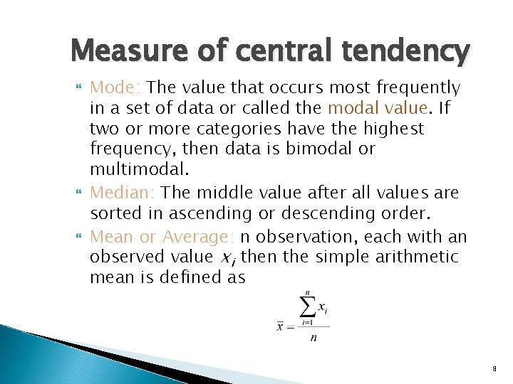
Measure of central tendency Mode: The value that occurs most frequently in a set of data or called the modal value. If two or more categories have the highest frequency, then data is bimodal or multimodal. Median: The middle value after all values are sorted in ascending or descending order. Mean or Average: n observation, each with an observed value xi then the simple arithmetic mean is defined as 8

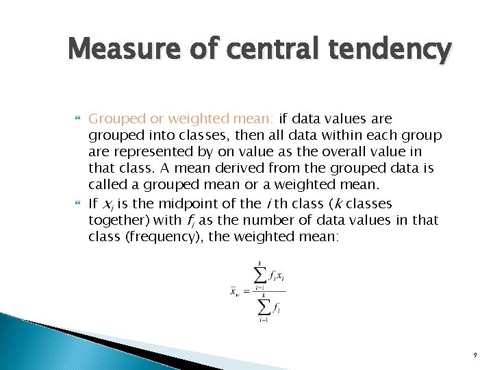
Measure of central tendency Grouped or weighted mean: if data values are grouped into classes, then all data within each group are represented by on value as the overall value in that class. A mean derived from the grouped data is called a grouped mean or a weighted mean. If xi is the midpoint of the i th class (k classes together) with fi as the number of data values in that class (frequency), the weighted mean: 9

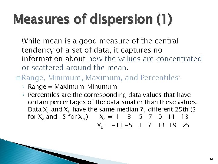
Measures of dispersion (1) While mean is a good measure of the central tendency of a set of data, it captures no information about how the values are concentrated or scattered around the mean. � Range, Minimum, Maximum, and Percentiles: ◦ Range = Maximum-Minumum ◦ Percentiles are the corresponding data values that have certain percentages of the data smaller than these values. Data Xa and Xb have the same median 7, different 25 th (3 for Xa and -5 for Xb ) Xa = 1 3 5 7 9 11 13 Xb = -11 -5 1 7 13 19 25 10

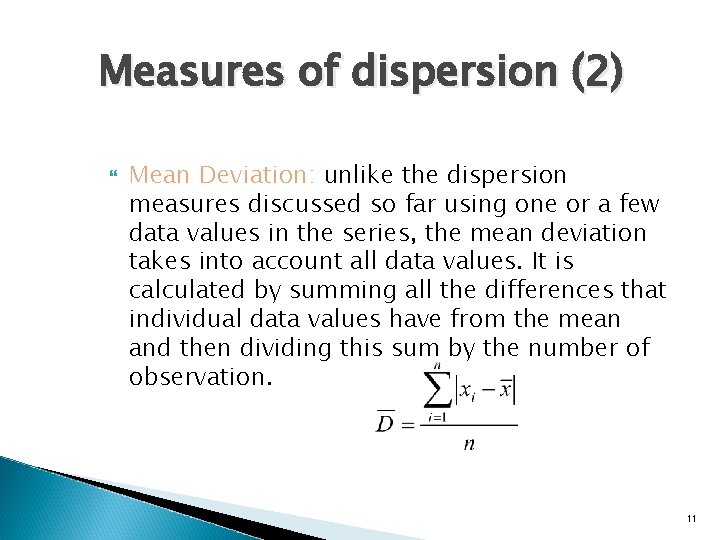
Measures of dispersion (2) Mean Deviation: unlike the dispersion measures discussed so far using one or a few data values in the series, the mean deviation takes into account all data values. It is calculated by summing all the differences that individual data values have from the mean and then dividing this sum by the number of observation. 11

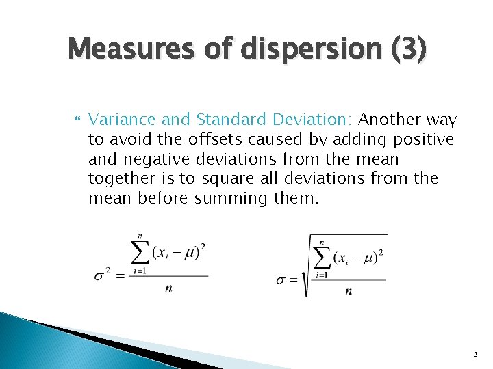
Measures of dispersion (3) Variance and Standard Deviation: Another way to avoid the offsets caused by adding positive and negative deviations from the mean together is to square all deviations from the mean before summing them. 12

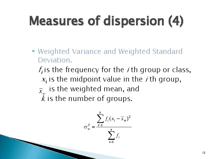
Measures of dispersion (4) Weighted Variance and Weighted Standard Deviation. fi is the frequency for the i th group or class, xi is the midpoint value in the i th group, is the weighted mean, and k is the number of groups. 13

Relationship Descriptors: Two Variables 14

One Variables � The mean and its variations address the issue of location, where the observations distribute along the continuous value line. Median and mode consider this central tendency issue. Variance, standard deviation, and percentiles address the issue of dispersion. Skewness deals with direction clustering. Kurtosis addresses the issue of concentration. All these measures focus on the distribution of the values using one variable at a time. 15

Relationship Descriptors � Mean, standard variable cannot measure the relationships between different distributions quantitatively. � One of statistics is based on the concept correlation measures statistically the direction and strength of the relationship between two sets of data or two variables for a number of observation. Regression measures the dependence of one variable on another. 16

Correlation Analysis (1) �Education is traditionally regarded as an asset. It enriches a person’s life in many ways. We usually believe that education and income are somewhat related and change in the same direction. If we recognize the value of education in eventually achieving a higher income, it would be nice to know how strong this relationship is, that is, how these aspects of life are related or correlated. 17

Correlation Analysis (2) � Each relationship has two important aspects: the direction and strength of the relationship. Between two related variable, the relationship is typically measured as correlation– a statistical measure indicating how values in one variable are related to values in the other variable. � Positive or direct correlation � Negative or inverse correlation 18

Trend Analysis �Trend analysis is a technique measuring the trend, while correlation is a statistical measure of two variables. �Trend analysis addresses the dependence of one variable on another. �Going beyond the strength and direction of the relationship, trend analysis allow us to model the relationship and to estimate likely value of one variable based on the value of another variable. �Models that are constructed with this technique are known as regression models. 19

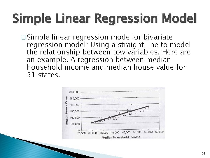
Simple Linear Regression Model � Simple linear regression model or bivariate regression model: Using a straight line to model the relationship between tow variables. Here an example. A regression between median household income and median house value for 51 states. 20

Regression model � Some phenomena may be modeled by the regression reasonable well, and others may not. � Regression model assumes a linear relationship between the variable. If the relationship is not linear or if the two variables have weak or no relationship, then the model will perform poorly. � A multivariate regression model, which can accommodate multiple independent variables. Under either circumstance, we may have committed a model specification error. 21

Point Pattern descriptors and analyzers 22

Point Pattern � Point Pattern Descriptors � Point Pattern Analyzers ◦ Central Tendency ◦ Dispersion and Orientation ◦ ◦ Quadrant Analysis Nearest-Neighbor Analysis Spatial Autocorrelation of Points K-Function 23

The Nature of Point Features Point pattern descriptors cover: �The methods for determining the overall patterns of a given set of points. �Measures used to describe the magnitude of spatial dispersion of a given set of points. �How the direction bias of a set of points can be extracted statistically. 24

Central Tendency of Point Distributions �A set of point descriptors provide certain descriptive information on the distribution of a set of points. � Central tendency information, mean centers, weighted mean centers, and median centers provide a good summary of how a set of points distributes in the geographic space. � To describe the spatial dispersion characteristics of a set of points, the measures of standard distance and standard ellipse will be discussed. These measures indicate the spatial variation and orientation of a point distribution. 25

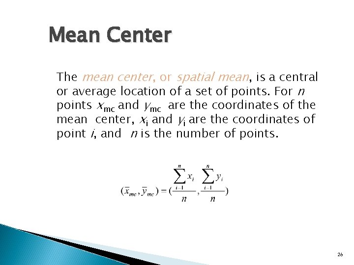
Mean Center The mean center, or spatial mean, is a central or average location of a set of points. For n points xmc and ymc are the coordinates of the mean center, xi and yi are the coordinates of point i, and n is the number of points. 26

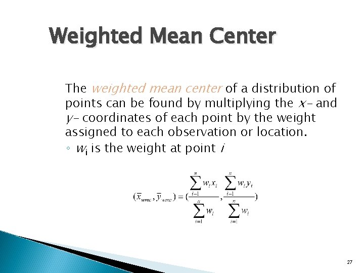
Weighted Mean Center The weighted mean center of a distribution of points can be found by multiplying the x- and y- coordinates of each point by the weight assigned to each observation or location. ◦ wi is the weight at point i 27

Dispersion and Orientation of Point Distributions � Two sets of points may occupy the same geographic space and may be interrelated. � For example, one set of points represents the location of forest fires and the other the locations of camping cabins in a wildlife region. They may have the same overall locations, but forest fire have a more dispersed spatial pattern than cabins. � In additional to spatial central tendency, it may be interesting to evaluate the magnitude of dispersion of locations and the orientation of the spatial distribution. 28

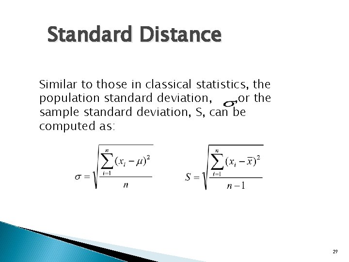
Standard Distance Similar to those in classical statistics, the population standard deviation, , or the sample standard deviation, S, can be computed as: 29

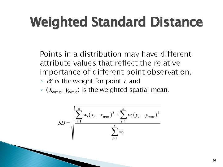
Weighted Standard Distance Points in a distribution may have different attribute values that reflect the relative importance of different point observation. ◦ Wi is the weight for point i, and ◦ (xwmc, ywmc) is the weighted spatial mean. 30

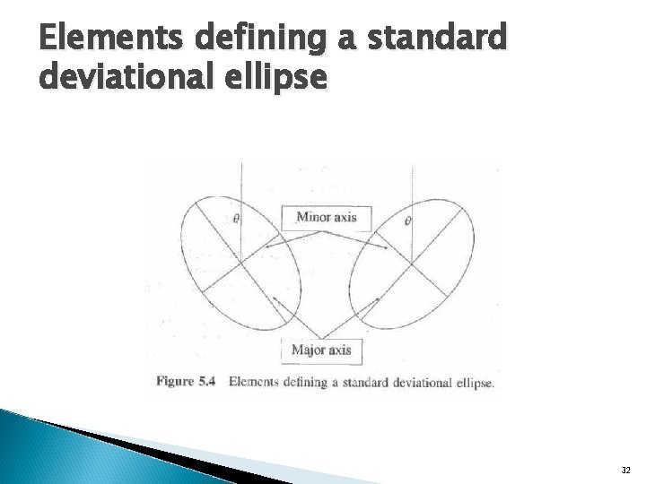
Standard Deviational Ellipses � The standard distance circle is a very effective visualization tool to show the spatial spread of a set of point location. �A logical extension of the standard distance circle is the standard deviational ellipse. It can capture the directional bias in a point distribution. Three components are needed to describe it: ◦ An angle of rotation ◦ Deviation along the major axis ◦ Deviation along the minor axis 31

Elements defining a standard deviational ellipse 32

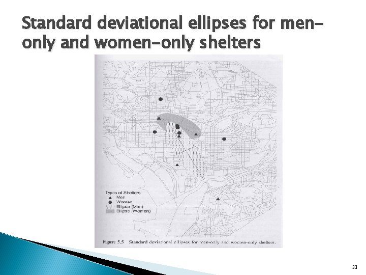
Standard deviational ellipses for menonly and women-only shelters 33

Point Pattern Analyzers � To fully understand the various states and dynamics of a particular geographic phenomenon, an analyst must be able to detect spatial patterns from the point distributions and to track the changes in point patterns at different time. 34

Point Pattern Analyzers � Quadrant Analysis allows analysts to determine if a point distribution is similar to a random pattern using a spatial sampling framework. � Nearest Neighbor Analysis compares the average distance between nearest neighbors in a set of points to that of a theoretical pattern. � Spatial autocorrelation coefficients measure how similar neighboring points are. � K-function analysis can identify and evaluate the clustering of points at different spatial scales, or extents. 35

Quadrant Analysis � Quadrant Analysis evaluates a point distribution by examining how its density changes over space. � The density measured by Quadrant Analysis is then compared with the density of a theoretically constructed random pattern to see if the point distribution in question is more clustered or more dispersed than the random pattern. 36

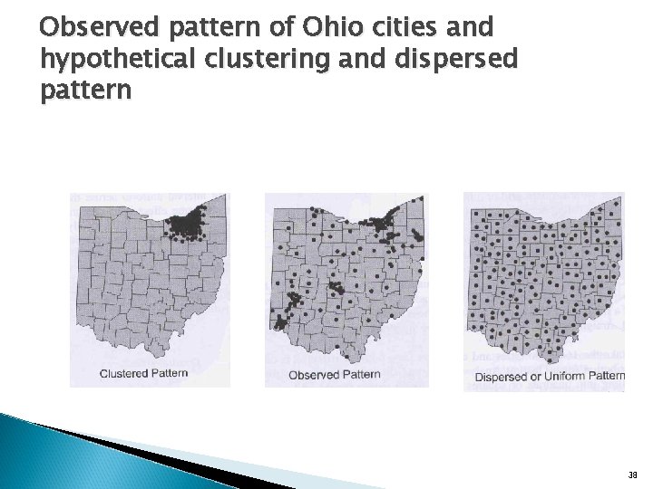
General Concept in Quadrant Analysis (1) A regular square grid and a number of points falling in some squares. � The square referred to as quadrants, which are essentially sampling units in spatial statistical jargon. � Circle is the most geometrically compact shape, however circles cannot cover the entire geographic space unless they overlap. � In an extremely clustered point pattern, all or most of the points fall inside one or a few squares only. In an extremely dispersed pattern referred to as a uniform pattern or a triangular lattice, all squares contain similar number of points. 37

Observed pattern of Ohio cities and hypothetical clustering and dispersed pattern 38

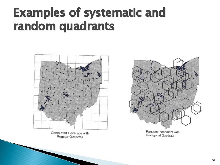
General Concept in Quadrant Analysis (2) � Statistically, Quadrant Analysis will achieve a fair evaluation of the density across the study area if it applies a large enough number of randomly generated quadrants. � An optimal size of quadrant can be calculated by 2 A/r. A is the area of study area, and r is the number of points in the distribution. � Once the quadrant size for a point distribution is determined, Quadrant Analysis can proceed to establish the frequency distribution of the number of points for all quadrant. 39

Examples of systematic and random quadrants 40

Comparing Observed and Expected Patterns Besides using K-S statistics to test if the observed pattern is different from a random pattern, one may perform the Variance. Mean Ratio Test by taking advantage of a specific statistical property of the Position distribution. 41

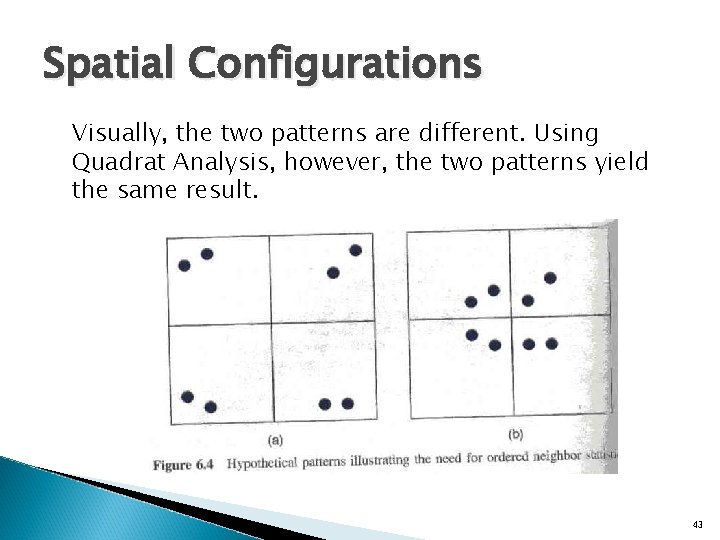
Ordered Neighbor Analysis �Quadrant Analysis is useful in comparing an observed point pattern to a random or theoretically known distribution. However, it has certain limitations. �The analysis captures information on the points within each quadrant, but no information on points between quadrants is used in the analysis. As a result, Quadrant Analysis may be insufficient to distinguish between certain point pattern in the following figures. 42

Spatial Configurations Visually, the two patterns are different. Using Quadrat Analysis, however, the two patterns yield the same result. 43

Nearest Neighbor Statistic � Nearest Neighbor Statistic is derived from the average distance between points and each of their nearest neighbors. � The second-ordered neighbor statistic uses the distance of the second nearest neighbors. Higherordered neighbors can be defined in similar ways. � Ordered Statistics can evaluate the pattern at different spatial scales. 44

Quadrant Analysis and Nearest Neighbor Analysis � While both Quadrant Analysis and Nearest Neighbor Analysis test point distribution, they utilize different spatial concepts. ◦ Quadrant Analysis tests a point distribution with the points per area concept using quadrants as sampling units. ◦ Nearest Neighbor Analysis uses the concept of area per point. �Both methods are similar in sense that the observed pattern is compared with some know distribution (random pattern). 45

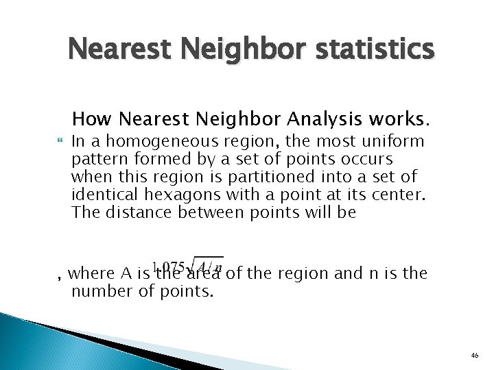
Nearest Neighbor statistics How Nearest Neighbor Analysis works. In a homogeneous region, the most uniform pattern formed by a set of points occurs when this region is partitioned into a set of identical hexagons with a point at its center. The distance between points will be , where A is the area of the region and n is the number of points. 46

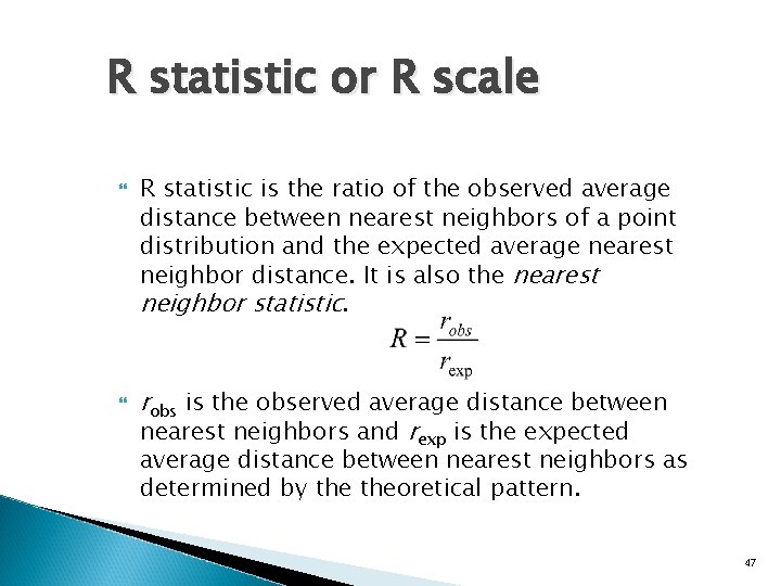
R statistic or R scale R statistic is the ratio of the observed average distance between nearest neighbors of a point distribution and the expected average nearest neighbor distance. It is also the nearest neighbor statistic. robs is the observed average distance between nearest neighbors and rexp is the expected average distance between nearest neighbors as determined by theoretical pattern. 47

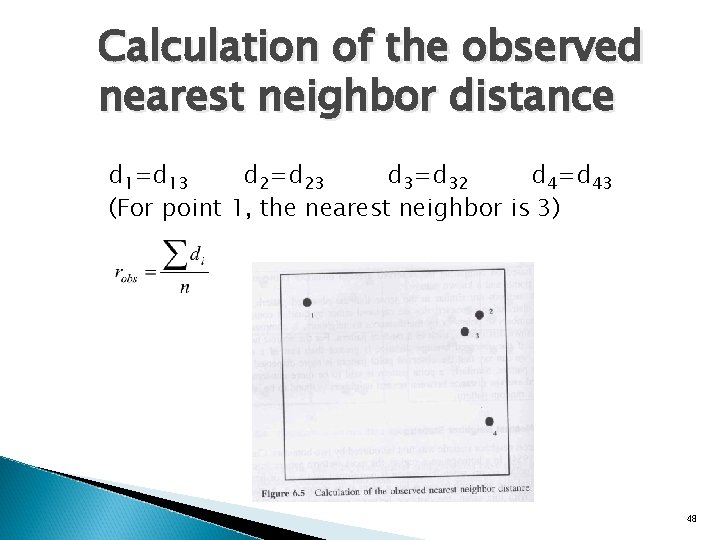
Calculation of the observed nearest neighbor distance d 1=d 13 d 2=d 23 d 3=d 32 d 4=d 43 (For point 1, the nearest neighbor is 3) 48

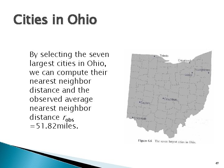
Cities in Ohio By selecting the seven largest cities in Ohio, we can compute their nearest neighbor distance and the observed average nearest neighbor distance robs =51. 82 miles. 49

Higher-order neighbor statistics � Nearest Neighbor Analysis has been extended to accommodate the second, third, and other higherorder neighbor definitions. When two points are not immediate nearest neighbors but rather the second nearest neighbors, the way distances are computed between them will need to be adjusted accordingly. 50

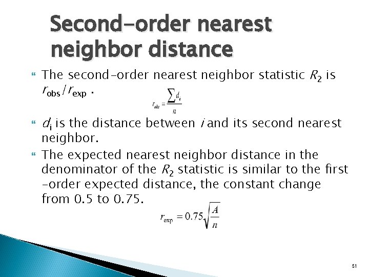
Second-order nearest neighbor distance The second-order nearest neighbor statistic R 2 is robs/rexp. di is the distance between i and its second nearest neighbor. The expected nearest neighbor distance in the denominator of the R 2 statistic is similar to the first -order expected distance, the constant change from 0. 5 to 0. 75. 51

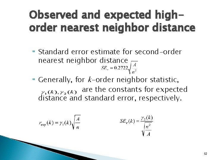
Observed and expected highorder nearest neighbor distance Standard error estimate for second-order nearest neighbor distance Generally, for k-order neighbor statistic, are the constants for expected distance and standard error, respectively. 52

K-Function Analysis Steps (1) Another statistic that can offer some insights and is more parsimonious to evaluate if the magnitude of clustering is uniform over different spatial scales is K-function analysis. It is an extension of the ordered neighbor statistics. For a set of point in a region, the K-function analysis involves following steps: � Select a distance increment or spatial lab, d, that is analogous to the unit reflecting the change in the spatial scale. � Set the iteration number g=1 to begin the process. 53

K-Function Analysis Steps (2) each point i in a region, create a circular buffer with a radius of h, where h=d*g. Therefore, the buffer will have a size d in the first iteration and 2 d in the second and so on. � For each point, count the number of points falling within its buffer of size h and denote that count as n(h). � Increase the radius of the buffer by d. � Repeat steps 3, 4, and 5 by increasing h until g=r or g=D/d. � Around 54

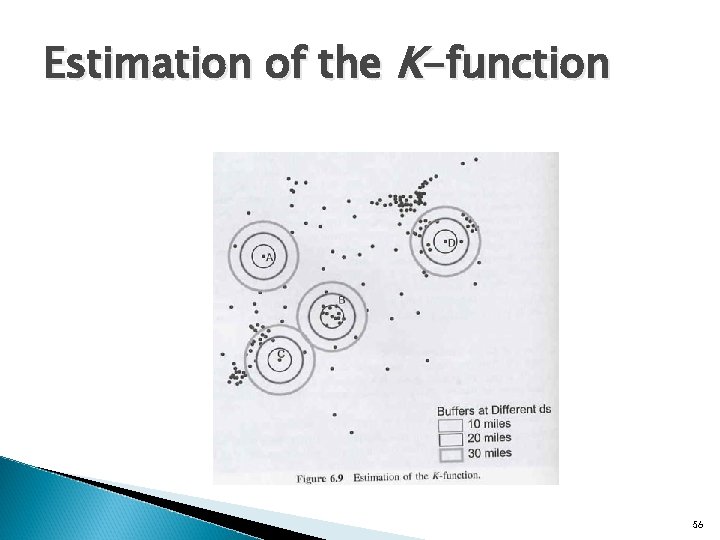
Estimation of the K-function Figure in next slide uses only four points to illustrate the procedure. ◦ Only three rings or buffers were created instead of the full range up to D. For a give h, we count the number of points within the buffers centered at all points. Point A is rather dispersed from other points, and therefore the counts are relatively low for buffers with small h. For point B, the point is in the middle of the cluster, and therefore the point count are relatively high with the small buffers, but the increases in point counts are substantial with large h’s. For Point C and D, the points themselves are apart from the cluster. 55

Estimation of the K-function 56

Relationship between point counts and the spatial lag h �The relationship between point counts and the spatial lag from empirical observation can be compared with a known patter, most likely a random pattern. �In a random pattern, point counts increase with increasing h but in no particular pattern. �K-function detect clustering at different scales by comparing the relationship between point counts and the size of h to that in a random distribution. 57

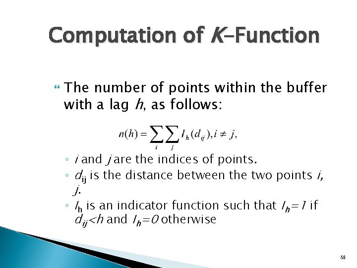
Computation of K-Function The number of points within the buffer with a lag h, as follows: ◦ i and j are the indices of points. ◦ dij is the distance between the two points i, j. ◦ Ih is an indicator function such that Ih=1 if dij<h and Ih=0 otherwise 58

Boundary Problems in K-Function � Sharing similar problems with other spatial statistical and analytical techniques, the K-function is also subject to the boundary problems. � Image that a point is located rather close to the edge of the study region. When buffers are formed around the point, a significant proportion of buffers will be outside of the study area and thus will distort the probability of finding a point within the vicinity of h. 59

Spatial Autocorrelation of Points � Spatial autocorrelation coefficients measure and test how clustered/dispersed the point locations are with respect to their attribute values. � Spatial autocorrelation of a set of points refers to the degree of similarity between points or events occurring at these points and points or evens in nearby locations. � With the spatial autocorrelation coefficient, we can measure: ◦ The proximity of location ◦ The similarity of the characteristics of these locations. 60

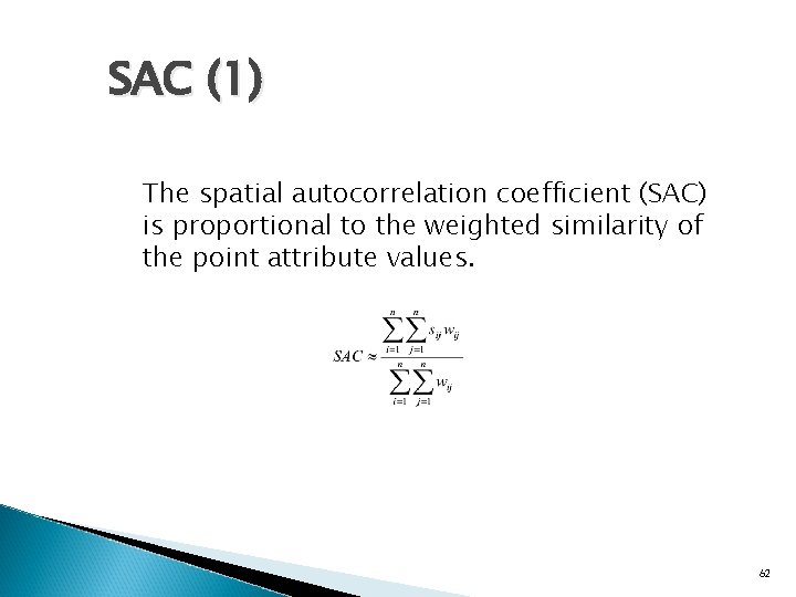
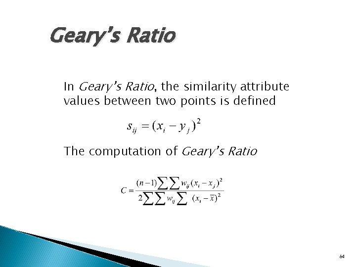
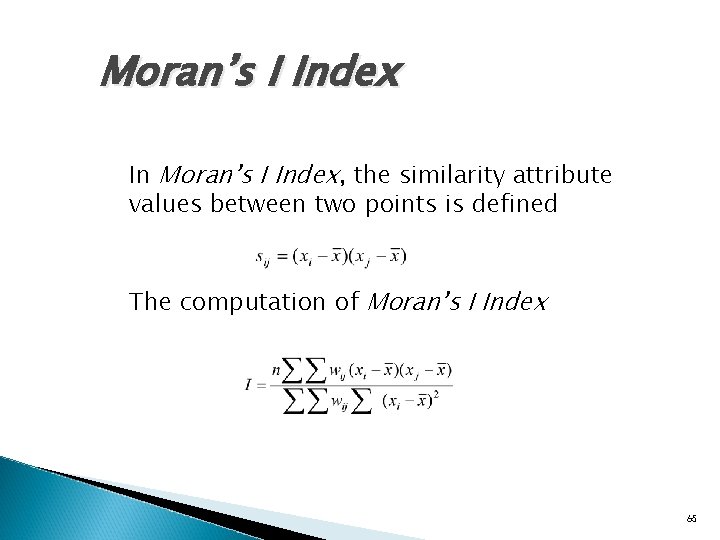
Measures for Spatial Autocorrelation Two popular indices for measuring spatial autocorrelation applicable to a point distribution: Geary’s Ratio and Moran’s I Index. � sij representing the similarity of point i ’s and point j ’s attributes. � wij representing the proximity of point i ’s and point j ’s locations, wii=0 for all points. � xi representing the value of the attribute of interest for point i. � n representing the total number of points. 61

SAC (1) The spatial autocorrelation coefficient (SAC) is proportional to the weighted similarity of the point attribute values. 62

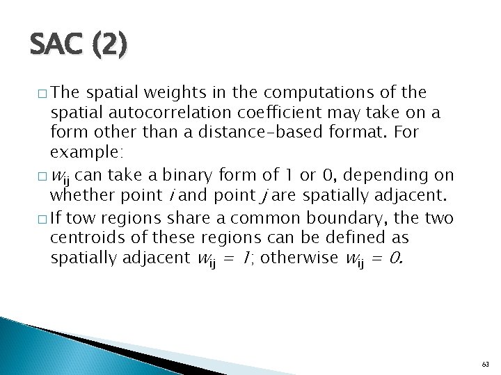
SAC (2) � The spatial weights in the computations of the spatial autocorrelation coefficient may take on a form other than a distance-based format. For example: � wij can take a binary form of 1 or 0, depending on whether point i and point j are spatially adjacent. � If tow regions share a common boundary, the two centroids of these regions can be defined as spatially adjacent wij = 1; otherwise wij = 0. 63

Geary’s Ratio In Geary’s Ratio, the similarity attribute values between two points is defined The computation of Geary’s Ratio 64

Moran’s I Index In Moran’s I Index, the similarity attribute values between two points is defined The computation of Moran’s I Index 65

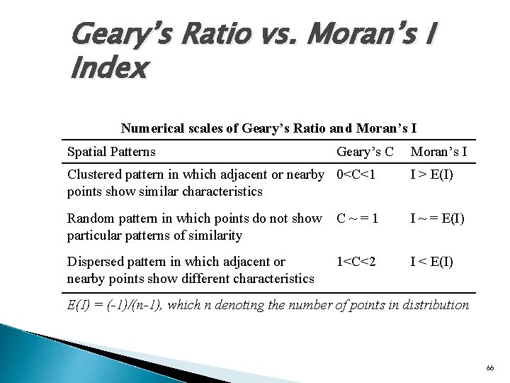
Geary’s Ratio vs. Moran’s I Index Numerical scales of Geary’s Ratio and Moran’s I Spatial Patterns Geary’s C Moran’s I Clustered pattern in which adjacent or nearby 0<C<1 points show similar characteristics I > E(I) Random pattern in which points do not show particular patterns of similarity C~=1 I ~ = E(I) Dispersed pattern in which adjacent or nearby points show different characteristics 1<C<2 I < E(I) = (-1)/(n-1), which n denoting the number of points in distribution 66

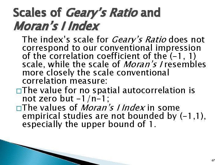
Scales of Geary’s Ratio and Moran’s I Index The index’s scale for Geary’s Ratio does not correspond to our conventional impression of the correlation coefficient of the (-1, 1) scale, while the scale of Moran’s I resembles more closely the scale conventional correlation measure: �The value for no spatial autocorrelation is not zero but -1/n-1; �The values of Moran’s I Index in some empirical studies are not bounded by (-1, 1), especially the upper bound of 1. 67

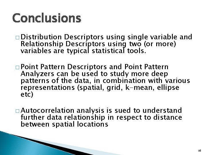
Conclusions � Distribution Descriptors usingle variable and Relationship Descriptors using two (or more) variables are typical statistical tools. � Point Pattern Descriptors and Point Pattern Analyzers can be used to study more deep patterns of the data, in combination with various representations (spatial, grid, k-mean, ellipse etc) � Autocorrelation analysis is sued to understand further data relationship in respect to distance between spatial locations 68