Statistical Alignment and Footprinting Rutgers DIMACS 27 4

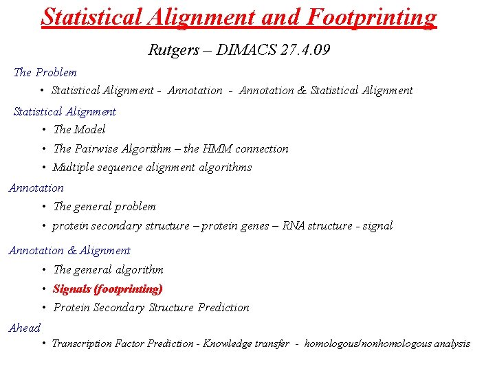
Statistical Alignment and Footprinting Rutgers – DIMACS 27. 4. 09 The Problem • Statistical Alignment - Annotation & Statistical Alignment • The Model • The Pairwise Algorithm – the HMM connection • Multiple sequence alignment algorithms Annotation • The general problem • protein secondary structure – protein genes – RNA structure - signal Annotation & Alignment • The general algorithm • Signals (footprinting) • Protein Secondary Structure Prediction Ahead • Transcription Factor Prediction - Knowledge transfer - homologous/nonhomologous analysis

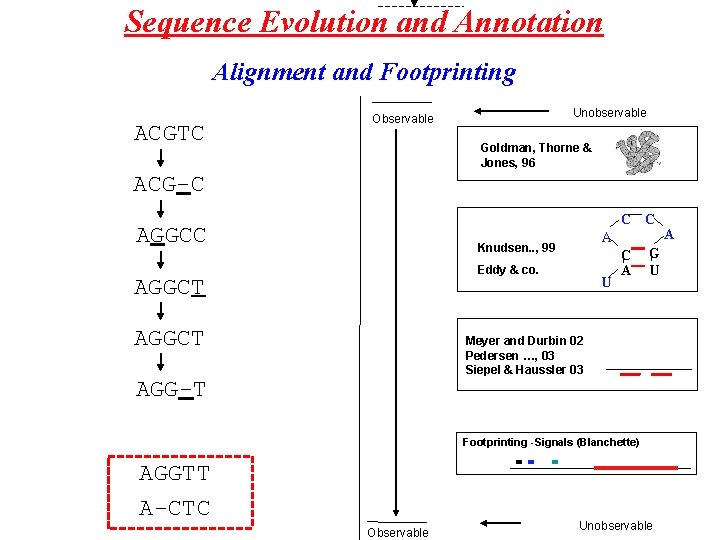
Sequence Evolution and Annotation Alignment and Footprinting ACGTC Unobservable Observable Goldman, Thorne & Jones, 96 ACG-C C C AGGCC A Knudsen. . , 99 Eddy & co. AGGCT U C A G U Meyer and Durbin 02 Pedersen …, 03 Siepel & Haussler 03 AGG-T Footprinting -Signals (Blanchette) AGGTT A-CTC Observable Unobservable A

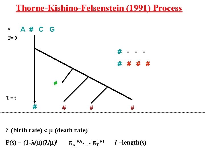
Thorne-Kishino-Felsenstein (1991) Process * A # C G T= 0 # - - # # # T=t # # l (birth rate) < m (death rate) P(s) = (1 -l/m)(l/m)l p. A #A*. . * p. T #T l =length(s)

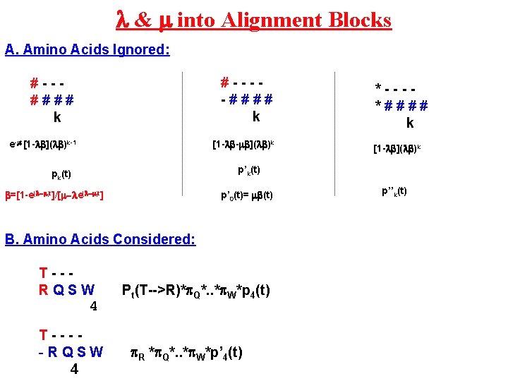
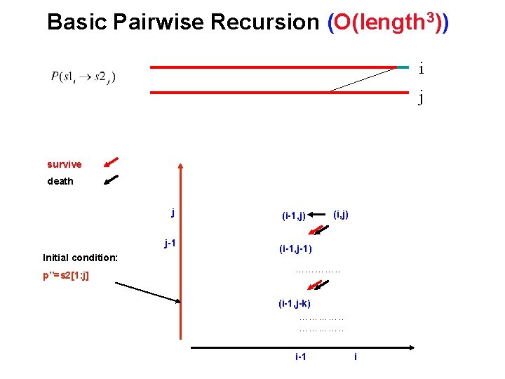
l & m into Alignment Blocks A. Amino Acids Ignored: #--#### k #----#### k e-mt[1 -lb](lb)k-1 [1 -lb-mb](lb)k b=[1 -e(l-m)t]/[m-le(l-m)t] p’ 0(t)= mb(t) B. Amino Acids Considered: T----RQSW 4 [1 -lb](lb)k p’k(t) pk(t) T--RQSW 4 *---*#### k Pt(T-->R)*p. Q*. . *p. W*p 4(t) p. R *p. Q*. . *p. W*p’ 4(t) p’’k(t)

Basic Pairwise Recursion (O(length 3)) i j survive death j j-1 Initial condition: p’’=s 2[1: j] (i-1, j) (i-1, j-1) …………. . (i-1, j-k) …………. . i-1 i

a-globin (141) and b-globin (146) (From Hein, Wiuf, Knudsen, Moeller & Wiebling 2000) a-globin VLSPADKTNVKAAWGKVGAHAGEYGAEALERMFLSFPTTKTYFPHFDLSHGSAQVKGHGKKVADALTNAVAH VDDMPNALSALSDLHAHKLRVDPVNFKLLSHCLLVTLAAHLPAEFTPAVHASLDKFLASVSTVLTSKYR b-globin VHLTPEEKSAVTALWGKVNVDEVGGEALGRLLVVYPWTQRFFESFGDLSTPDAVMGNPKVKAHGKKVLGAFS DGLAHLDNLKGTFATLSELHCDKLHVDPENFRLLGNVLVCVLAHHFGKEFTPPVQAAYQKVVAGVANALAHK YH l*t: m*t: s*t: 430. 108 327. 320 747. 428 0. 0371805 +/- 0. 0135899 0. 0374396 +/- 0. 0136846 0. 91701 +/- 0. 119556 : -log(a-globin) : -log(a-globin --> b-globin) : -log(a-globin, b-globin) = -log(l(sumalign)) Maximum contributing alignment: V-LSPADKTNVKAAWGKVGAHAGEYGAEALERMFLSFPTTKTYFPHF-DLS--H---GSAQVKGHGKKVADALT VHLTPEEKSAVTALWGKV--NVDEVGGEALGRLLVVYPWTQRFFESFGDLSTPDAVMGNPKVKAHGKKVLGAFS NAVAHVDDMPNALSALSDLHAHKLRVDPVNFKLLSHCLLVTLAAHLPAEFTPAVHASLDKFLASVSTVLTSKYR DGLAHLDNLKGTFATLSELHCDKLHVDPENFRLLGNVLVCVLAHHFGKEFTPPVQAAYQKVVAGVANALAHKYH Ratio l(maxalign)/l(sumalign) = 0. 00565064

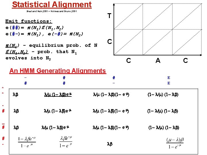
Statistical Alignment Steel and Hein, 2001 + Holmes and Bruno, 2001 T Emit functions: e(##)= p(N 1)f(N 1, N 2) e(#-)= p(N 1), e(-#)= p(N 2) p(N 1) - equilibrium prob. of N C f(N 1, N 2) - prob. that N 1 evolves into N 2 C An HMM Generating Alignments # # - E E * * lb l/m (1 - lb)e-m l/m (1 - lb)(1 - e-m) (1 - l/m) (1 - lb) # lb l/m (1 - lb)e-m l/m (1 - lb)(1 - e-m) (1 - l/m) (1 - lb) _ # lb l/m (1 - lb)(1 - e-m) (1 - l/m) (1 - lb) # - l/m (1 - lb)e-m lb

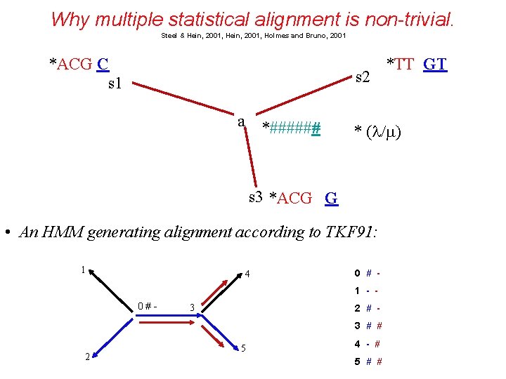
Why multiple statistical alignment is non-trivial. Steel & Hein, 2001, Holmes and Bruno, 2001 *ACG C s 1 s 2 a *###### * (l/m) s 3 *ACG G • An HMM generating alignment according to TKF 91: 1 4 0 # 1 - - 0#- 3 2 # 3 # # 2 5 *TT GT 4 - # 5 # #

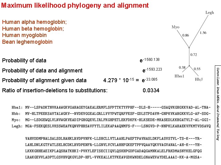
Maximum likelihood phylogeny and alignment Human alpha hemoglobin; Human beta hemoglobin; Human myoglobin Bean leghemoglobin Probability of data e -1560. 138 Probability of alignment given data e -1593. 223 4. 279 * 10 -15 = e-33. 085 Ratio of insertion-deletions to substitutions: 0. 0334 Gerton Lunter, Istvan Miklos, Alexei Drummond, Yun Song Probability of data and alignment

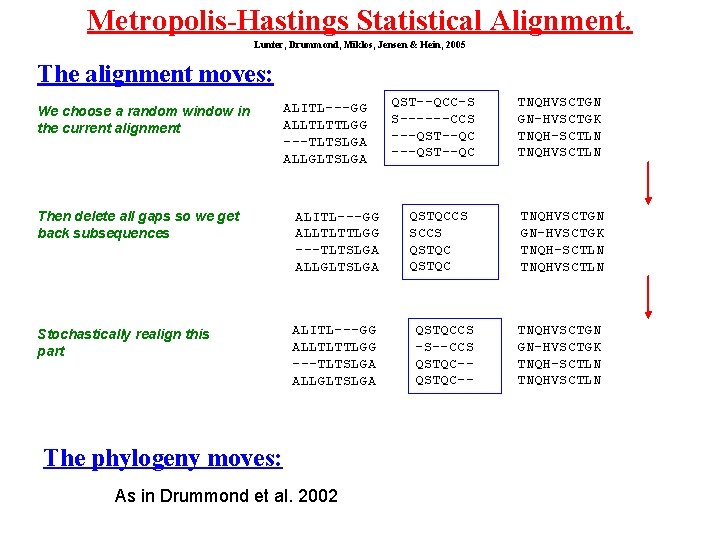
Metropolis-Hastings Statistical Alignment. Lunter, Drummond, Miklos, Jensen & Hein, 2005 The alignment moves: We choose a random window in the current alignment ALITL---GG ALLTLTTLGG ---TLTSLGA ALLGLTSLGA Then delete all gaps so we get back subsequences ALITL---GG ALLTLTTLGG ---TLTSLGA ALLGLTSLGA Stochastically realign this part ALITL---GG ALLTLTTLGG ---TLTSLGA ALLGLTSLGA The phylogeny moves: As in Drummond et al. 2002 QST--QCC-S S------CCS ---QST--QC QSTQCCS SCCS QSTQCCS -S--CCS QSTQC-- TNQHVSCTGN GN-HVSCTGK TNQH-SCTLN TNQHVSCTLN

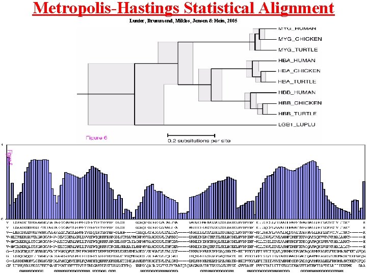
Metropolis-Hastings Statistical Alignment Lunter, Drummond, Miklos, Jensen & Hein, 2005

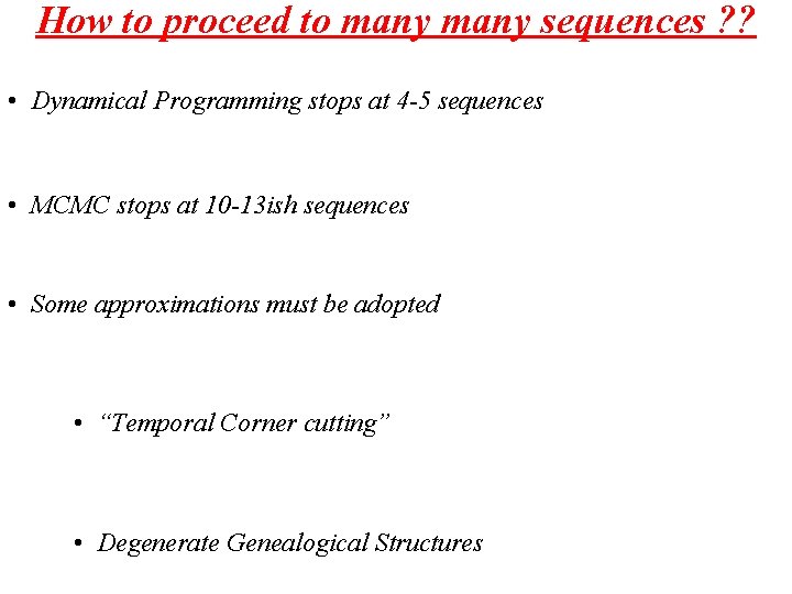
How to proceed to many sequences ? ? • Dynamical Programming stops at 4 -5 sequences • MCMC stops at 10 -13 ish sequences • Some approximations must be adopted • “Temporal Corner cutting” • Degenerate Genealogical Structures

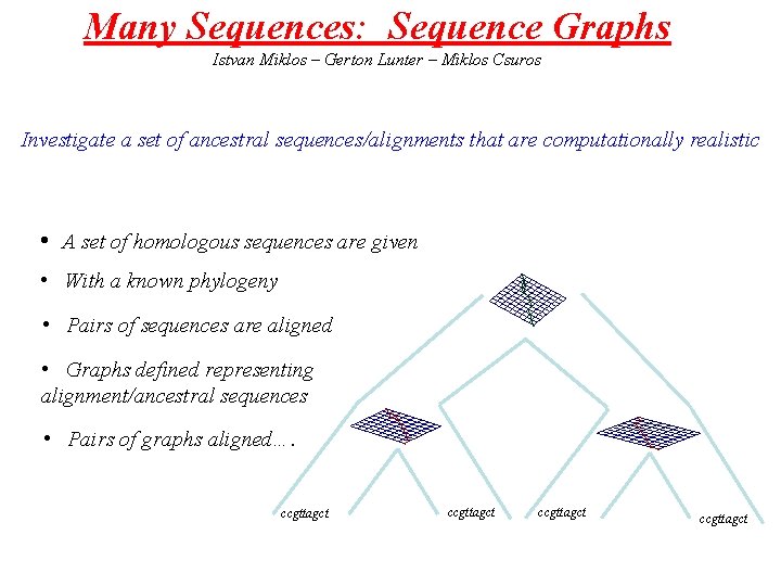
Many Sequences: Sequence Graphs Istvan Miklos – Gerton Lunter – Miklos Csuros Investigate a set of ancestral sequences/alignments that are computationally realistic • A set of homologous sequences are given • With a known phylogeny • Pairs of sequences are aligned • Graphs defined representing alignment/ancestral sequences • Pairs of graphs aligned…. ccgttagct

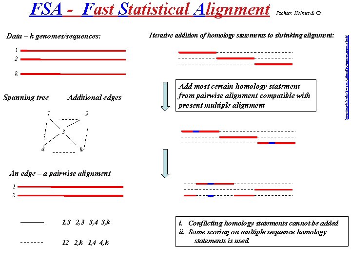
Data – k genomes/sequences: Pachter, Holmes & Co Iterative addition of homology statements to shrinking alignment: 1 2 k Spanning tree Additional edges 1 Add most certain homology statement from pairwise alignment compatible with present multiple alignment 2 3 4 k An edge – a pairwise alignment 1 2 1, 3 2, 3 3, 4 3, k 12 2, k 1, 4 4, k i. Conflicting homology statements cannot be added ii. Some scoring on multiple sequence homology statements is used. http: //math. berkeley. edu/~rbradley/papers/manual. pdf FSA - Fast Statistical Alignment

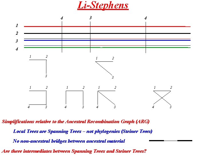
Li-Stephens 3 4 4 1 2 3 1 4 3 1 2 3 4 Simplifications relative to the Ancestral Recombination Graph (ARG) Local Trees are Spanning Trees – not phylogenies (Steiner Trees) No non-ancestral bridges between ancestral material Are there intermediates between Spanning Trees and Steiner Trees? 2 3

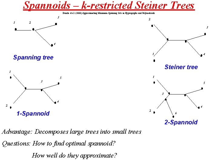
Spannoids – k-restricted Steiner Trees Baudis et al. (2000) Approximating Minimum Spanning Sets in Hypergraphs and Polymatroids 3 1 2 2 3 4 1 Spanning tree 4 Steiner tree 1 1 5 3 4 2 4 1 -Spannoid 2 6 2 -Spannoid Advantage: Decomposes large trees into small trees Questions: How to find optimal spannoid? How well do they approximate?

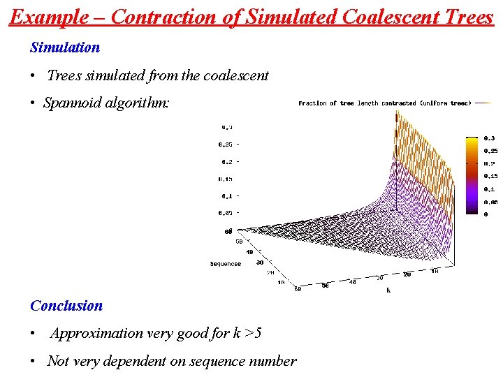
Example – Contraction of Simulated Coalescent Trees Simulation • Trees simulated from the coalescent • Spannoid algorithm: Conclusion • Approximation very good for k >5 • Not very dependent on sequence number

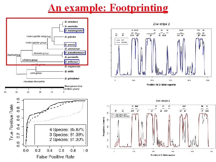
Annotation & Annotation with alignment • Annotation and alignment • Footprinting • Three Programs • SAPF – dynamic programming up to 4 sequences • Big. Foot– MCMCup to 13 sequences • GRAPEfoot – pairwise genome footprinting

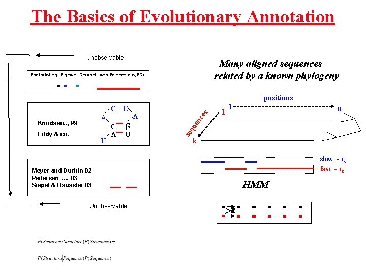
The Basics of Evolutionary Annotation Unobservable Many aligned sequences related by a known phylogeny Footprinting -Signals (Churchill and Felsenstein, 96) Eddy & co. U C A G U Meyer and Durbin 02 Pedersen …, 03 Siepel & Haussler 03 Unobservable A 1 1 n qu A Knudsen. . , 99 se C C en ce s positions k slow - rs fast - rf HMM

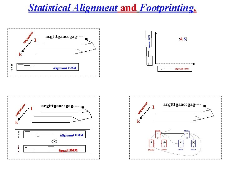
1 acgtttgaaccgag---- Structure HMM se qu en c es Statistical Alignment and Footprinting. (A, S) k ce s acgtttgaaccgag---- en 1 Alignment HMM se qu en ce s Alignment HMM k k Alignment HMM Signal HMM 1 acgtttgaaccgag----

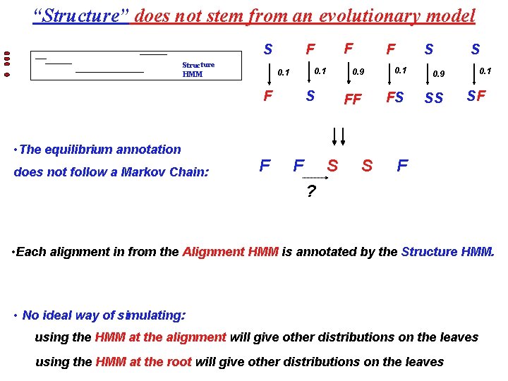
“Structure” does not stem from an evolutionary model S Structure HMM 0. 1 F • The equilibrium annotation does not follow a Markov Chain: F F F 0. 9 S F F FF S S S 0. 1 0. 9 FS SS S 0. 1 SF F ? • Each alignment in from the Alignment HMM is annotated by the Structure HMM. • No ideal way of simulating: using the HMM at the alignment will give other distributions on the leaves using the HMM at the root will give other distributions on the leaves

An example: Footprinting

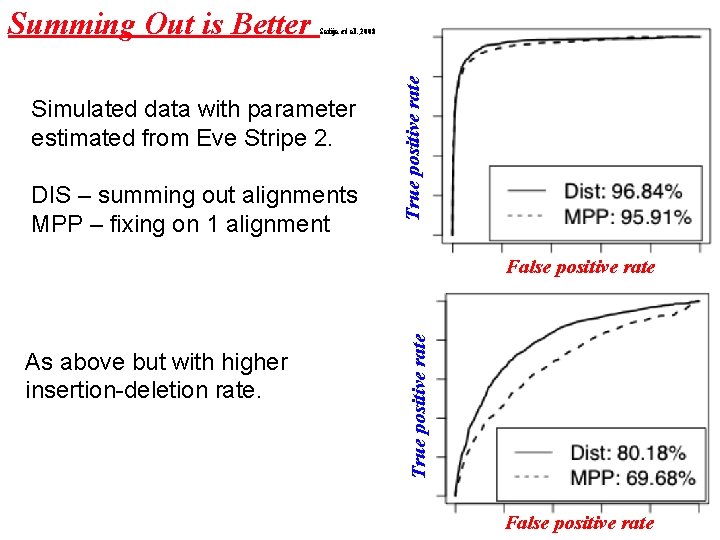
Satija et al. , 2008 Simulated data with parameter estimated from Eve Stripe 2. DIS – summing out alignments MPP – fixing on 1 alignment True positive rate Summing Out is Better As above but with higher insertion-deletion rate. True positive rate False positive rate

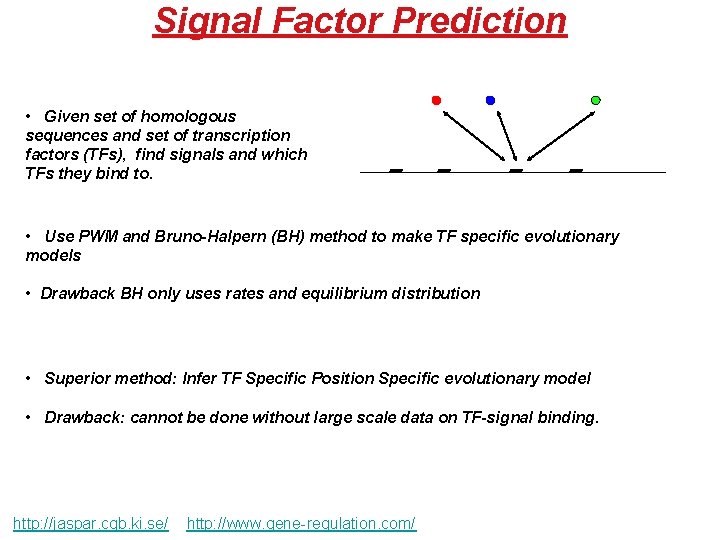
Signal Factor Prediction • Given set of homologous sequences and set of transcription factors (TFs), find signals and which TFs they bind to. • Use PWM and Bruno-Halpern (BH) method to make TF specific evolutionary models • Drawback BH only uses rates and equilibrium distribution • Superior method: Infer TF Specific Position Specific evolutionary model • Drawback: cannot be done without large scale data on TF-signal binding. http: //jaspar. cgb. ki. se/ http: //www. gene-regulation. com/

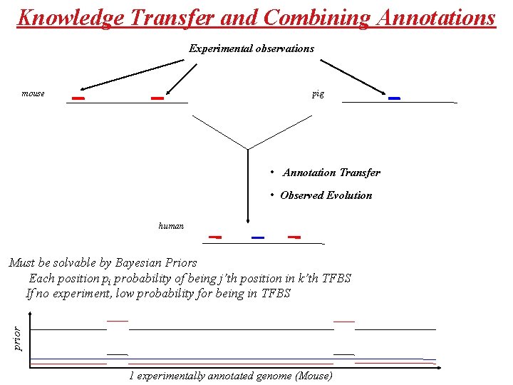
Knowledge Transfer and Combining Annotations Experimental observations mouse pig • Annotation Transfer • Observed Evolution human prior Must be solvable by Bayesian Priors Each position pi probability of being j’th position in k’th TFBS If no experiment, low probability for being in TFBS 1 experimentally annotated genome (Mouse)

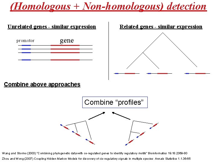
(Homologous + Non-homologous) detection Unrelated genes - similar expression promotor Related genes - similar expression gene Combine above approaches Combine “profiles” Wang and Stormo (2003) “Combining phylogenetic data with co-regulated genes to identify regulatory motifs” Bioinformatics 19. 18. 2369 -80 Zhou and Wong (2007) Coupling Hidden Markov Models for discovery of cis-regulatory signals in multiple species Annals Statistics 1. 1. 36 -65

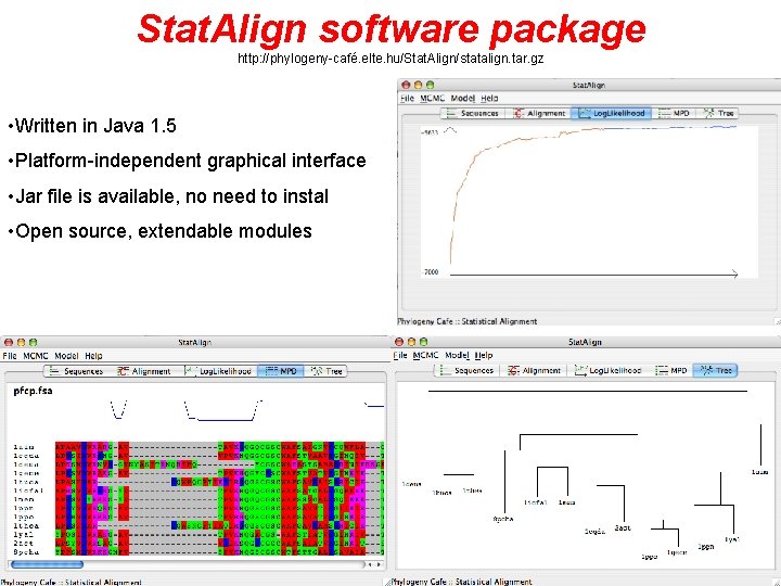
Stat. Align software package http: //phylogeny-café. elte. hu/Stat. Align/statalign. tar. gz • Written in Java 1. 5 • Platform-independent graphical interface • Jar file is available, no need to instal • Open source, extendable modules

Summary The Problem • Statistical Alignment - Annotation & Statistical Alignment • The Model • The Pairwise Algorithm – the HMM connection • the multiple sequence alignment algorithm Annotation • The general problem • protein secondary structure – protein genes – RNA structure - signal Annotation & Alignment • The general algorithm • Signals (footprinting) • Protein Secondary Structure Prediction Ahead • Transcription Factor Prediction - Knowledge transfer - homologous/nonhomologous analysis

Acknowledgements Footprinting: Rahul Satija, Lior Pachter, Gerton Lunter MCMC: Istvan Miklos, Jens Ledet Jensen, Alex Drummond, Program: Adam Novak, Rune Lyngsø Spannoids: Jesper Nielsen, Christian Storm Earlier Statistical alignment Collaborators Mike Steel, Yun Song, Carsten Wiuf, Bjarne Knudsen, Gustav Wiebling, Christian Storm, Morten Møller, Funding BBSRC MRC Rhodes Foundation Software http: //phylogeny-café. elte. hu/Stat. Align/statalign. tar. gz Next steps http: //www. stats. ox. ac. uk/research/genome/projects

Statistical Aligment and Footprinting Statistical Alignment and Footprinting Although bioinformatics perceived is a new discipline, certain parts have a long history and could be viewed as classical bioinformatics. For example, application of string comparison algorithms to sequence alignment has a history spanning the last three decades, beginning with the pioneering paper by Needleman and Wunch, 1970. They used dynamic programming to maximize a similarity score based on a cost of insertion-deletions and a score function on matched amino acids. The principle of choosing solutions by minimizing the amount of evolution is also called parsimony and has been widespread in phylogenetic analysis even if there is no alignment problem. This situation is likely to change significantly in the coming years. After a pioneering paper by Bishop and Thompson (1986) that introduced and approximated likelihood calculation, Thorne, Kishino and Felsenstein (1991) proposed a well defined time reversible Markov model for insertion and deletions (the TKF 91 -model), that allowed a proper statistical analysis for two sequences. Such an analysis can be used to provide maximum likelihood (pairwise) sequence alignments, or to estimate the evolutionary distance between two sequences. Steel et al. (2001) generalized this to any number of sequences related by a star tree. This was subsequently generalized further to any phylogeny and more practical methods based on MCMC has been developed. We have developed this into a generally available program package. Traditional alignment-based phylogenetic footprinting approaches make predictions on the basis of a single assumed alignment. The predictions are therefore highly sensitive to alignment errors or regions of alignment uncertainty. Alternatively, statistical alignment methods provide a framework for performing phylogenetic analyses by examining a distribution of alignments. We developed a novel algorithm for predicting functional elements by combining statistical alignment and phylogenetic footprinting (SAPF). SAPF simultaneously performs both alignment and annotation by combining phylogenetic footprinting techniques with an hidden Markov model (HMM) transducer-based multiple alignment model, and can analyze sequence data from multiple sequences. We assessed SAPF's predictive performance on two simulated datasets and three well-annotated cis-regulatory modules from newly sequenced Drosophila genomes. The results demonstrate that removing the traditional dependence on a single alignment can significantly augment the predictive performance, especially when there is uncertainty in the alignment of functional regions. The transducer-based version of SAPF is currently able to analyze data from up to five sequences. We are currently developing an MCMC approach that we hope will be capable of analyzing data from 12 -16 species, enabling the user to input sequence data from all 12 recently sequenced Drosophila genomes. We will present initial results from the MCMC version of SAPF and discuss some of the challenges and difficulties affecting the speed of convergence.