Static Equilibrium Asset Pricing Chapter 3 Capital Asset

Static Equilibrium Asset Pricing Chapter 3
 Section 3. 1")
Capital Asset Pricing Model (CAPM) Section 3. 1

CAPM • • Original portfolio-based asset pricing model Most all modern asset pricing builds from this Sharpe/Lintner (and sort of Treynor) 1960’s Assumptions • • All investors price takers Common information/beliefs Portfolios evaluated on means and variances Pick some mean/variance efficient portfolio • Equilibrium • Market portfolio = tangent portfolio • Market portfolio is mean/var efficient • At market price (return) equilibrium, no way to better mean/var asset portfolio

CAPM with risk free
")
Portfolio change experiment (should look familiar from micro)

Guts of CAPM • This isn’t very testable • Assume market portfolio is MV efficient

CAPM regression
 Section 3. 1. 2")
Black CAPM (borrowing constraints) Section 3. 1. 2

Risk free rates • • Assume lending, but no borrowing This can get much more complex in terms of rates We are just glancing at this quickly People vary in their risk preferences (risky portfolios now differ) • Assume all portfolios on frontier • All portfolios are weighted sums of two fixed mutual funds (separation) • This implies that the market portfolio is also a weighted sum of these and lies on the frontier itself • Can yield a CAPM, but risk free replaced with “zero beta” portfolio • The key idea here is that the existence of a risk free asset is not critical to a CAPM like beta pricing relationship

Black CAPM

CAPM Applications in real portfolios Section 3. 1. 3

Harvard endowment portfolios through time
")
Sharpe ratios (market = line)

Security market line

Last figures • These last two figures are important in relation to the CAPM • The CAPM makes no statement about where individual returns sit relative to their standard deviation (Sharpe ratios) • The Sharpe ratio does define the slope of the line through the tangent (and often market) portfolio • The CAPM does make a strong statement about the slope of the line in the second figure (The Security Market line) • Expected returns of all portfolios should lie on this line • Some tests of the CAPM statistically test the “distance” of returns from the SML • Active manager strive to achieve “alpha” which puts them above this line

Investment management • The CAPM also says a lot of about performance and investment management • Investors should not “pay for beta risk” • If an investment manager delivers a higher expected return, but is still on the SML (zero alpha), investors could just do this themselves by borrowing (leverage) and buying more of the market • This does also correspond to moving out beyond the tangent portfolio in the std/return plots too • Why pay someone for something you can do yourself • This intuition will carry over into our logic for arbitrage pricing

A simple picture of return/beta from Malkiel and Fama/French
 • Standard portfolio selection generates “crazy” portfolio weights • Noise")
Black/Litterman CAPM (casual description) • Standard portfolio selection generates “crazy” portfolio weights • Noise in expected returns creates big swings in weights • Black/Litterman • Set a kind of prior for returns that follow a standard CAPM • W considers how strong beliefs are in current sample estimates versus CAPM prior • Fed into standard portfolio optimization • Black/Litterman sort of casual (see book) • This is a form of empirical Bayes estimation

Multifactor models/Arbitrage Pricing Section 3. 2. 1

Thoughts on arbitrage • Key concept in finance • Portfolios that generate same payoffs should have same price • Very powerful • Does not rely on preferences • Can sometimes be limited in scope • Examples • Arbitrage Pricing Theory (APT) • Black/Scholes • Much of fixed income pricing
 • Few assumptions about")
Arbitrage pricing • Important model • And modeling style (arbitrage) • Few assumptions about preferences • Related to other models such as Black/Scholes • Also, related to CAPM, and modern multi-factor (Fama/French) factor models

Excess return and zero cost strategies • We often state stuff in terms of excess returns • They have many convenient features • One is that investors can add any excess return to a portfolio with no concern for budgets • They are “zero cost” investments • Increase risky asset, borrow risk free

APT factor structure
 units of the market portfolio")
Basic arbitrage • Buy portfolio • Then short (allowed) units of the market portfolio • This will give you a completely risk free payout • Absence of arbitrage implies these free lunches do not exist • Therefore, • What about for individual securities?

Individual securities • This does not say that each alpha is zero • This depends on thinking about N big, and lots of securities • If there are groups where alpha is big then • Buy them • Neutralize market risk • Take arbitrage profits • Alpha for individuals must stay close to zero

Technical aside • Does this imply: • No, this is only a limiting result • Some of these expected returns might be nonzero, but they generally need to be “pretty small” • This can get technical fast • See Campbell (pp 56 -57) for proof that APT implies that: • Proof is not super difficult, but will skip

What else can screw up for APT? • Factor structure not correct • Other factors • Idiosyncratic errors not independent • This is a problem • You need to be able to build the diversified factor portfolios that let you ignore idiosyncratic risk • This is related to the “other factors” issue

Multifactor models Section 3. 2. 2

Multiple factor structure
 structure (like CAPM) • MV efficient set is")
Implications • Linear pricing (expected returns) structure (like CAPM) • MV efficient set is spanned by K factor portfolios • Why? • Think about portfolio on frontier with some idiosyncratic risk • One could replicate this exactly in terms of expected returns and systematic risk (factor risk) by purchasing factor portfolios • This would have same expected return and smaller variance • So no portfolio exists on the frontier that we can’t do better using pure factor returns • Practical aside: • Some factor portfolios can be directly purchased as exchange traded funds (ETF’s)

Empirical history of APT • Principle components • Macro factors • Portfolio factors • This has been the most successful

Conditional CAPM and factors Section 3. 2. 3

Conditional CAPM and multifactors • A conditional CAPM can be mapped into a multifactor model • Allow beta to move around through time • This is now a two factor model • Factor 2 is the market return “scaled” by info variable z(t) • This is a kind of synthetic strategy which increases/decreases market holdings depending on z(t)
 Section 3. 3. 1 Test methodology")
Empirical evidence (light) Section 3. 3. 1 Test methodology

CAPM: Three basic tests • Time series • Cross sectional • Fama/Mac. Beth

Time series approach • Could run for one security, and test alpha=0 • Joint tests for alpha(i)=0 • Assume errors iid • Asymptotic Chi-squared test on weighted squared alpha (3. 45) • Adjusts for beta uncertainty in model • Finite sample F-test (3. 46) • Distance of market Sharpe ratio from tangency Sharpe ratio

Cross-sectional approach • Estimate beta’s from time series regressions • Then run cross-section regression (no intercept) • This is again a chi-squared test • Estimation needs GLS (a’s not independent/cross sectional dependence) • Asymptotic test statistic (3. 51)
 • Cross-section with time series changes • Useful test • Used outside")
Fama-Mac. Beth(1973) • Cross-section with time series changes • Useful test • Used outside of finance too (rolling cross sectional) • Method: • Run time series regression to get Beta’s • Then cross-sectional regression at each time t • FM get standard errors • Problem: Does not adjust for beta estimation • Interesting: Can be done with changing beta’s
 • Estimate beta in window •")
Rolling Fama/Mac. Beth • Set window (1, T) • Estimate beta in window • Estimate CAPM in T+1 • Set window (2, T+1) • Estimate beta in window • Estimate CAPM T+2

Returns and characteristics • Cross sectional F/M useful for adding other things to CAPM testing • In true CAPM world other stuff should not matter • Many flavors of this • X can be any firm level characteristic (profits, growth, size) • Drop beta • More factors • Trading strategy interpretation (see 3. 55)

Choosing test assets • Occasionally individual stocks are grouped into portfolios for testing • All asset pricing theory should hold for portfolios • For example “high beta” and “low beta” portfolios replace R(it) • Designed to get more power/precision in tests • Can be controversial (see references on p 66)

Empirical features Section 3. 3. 2

Individual asset return time series features • Nearly uncorrelated • Prices near random walk • Non normal distributions at frequencies less than quarterly • Persistent volatility • Increasing when prices fall (Leverage effect) • Most of academic research is on cross-sectional features • This is where AP models operate

CAPM • Early tests in 1970’s • Works but, • Beta small • Barely significant • Working less well after 1960 • Remember Malkiel picture
 • Smaller firms have higher returns •")
Size • Size = market capitalization (shares*price) • Smaller firms have higher returns • Often in the month of January • The “January effect” • See next figure • Note: portfolio sort technology

Size portfolios
, Buffet) • Key ratio (something)/(market cap)")
Value • Extremely old strategy (Graham, Dodd, Cottle(1934), Buffet) • Key ratio (something)/(market cap) • Something = book value, dividends, earnings • High ratio • Cheap stocks • Buy!!

Value sorts

Momentum • Persistence in returns • Autocorrelations are a little more subtle than zero • Negative at highest (intraday/daily) frequencies • Positive at mid range (monthly-yearly) • Strategy: Buy recent winners • Negative (reversals) at long horizons (5 years) • Strategy: Buy losers

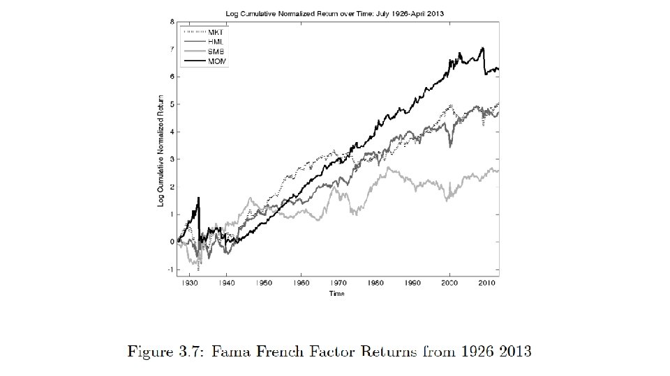
Modern research midrange • Formation period • • Previous 6 -12 months Sort (maybe 5 -10 portfolios) based on returns in this period Wait 1 month Strategy test in next month after this • Long winner portfolio, short loser • Several different flavors of this • All strategies together (next figure) • MOM • SMB (small minus big, size) • HML (book/market, value) • Much of this data is available at Ken French’s website

More features • Post-event drift • Turnover/volatility • Idiosyncratic risk negative with future returns • This is weird for many reasons • Insider trading • Growth • Earnings and accounting • Profitability • A predictor zoo?

Some response to this • Data mining • Some of these results not real • Mined from data • See Harvey(2017, JF) • Anomaly elimination • Mc. Lean/Pontiff(2016, JF) • Many features change/disappear after they become well known
")
Small stocks (Jan versus other months)

Roll critique • Don’t observe the true market portfolio • Creative expansion on what market portfolio is • Should include human capital? ? • CAPM is untestable? • Further problems in macro/finance • Consumption/wealth ratios • Doesn’t apply to the APT
 • Conditional CAPM • Expand beta’s in")
Other issues • Illiquidity (see chapter 12) • Conditional CAPM • Expand beta’s in conditioning information (3. 41 -43) • Some success, but no major solutions • What is the conditioning information? • More stability and data mining issues

The Four Factor Model • Modern work horse empirical model • Fama/French, Carhart • Four portfolio based factors • • Market – risk free Small – large stocks High book/market – low book market MOM: recent winners-losers • Estimate betas on these factors • Estimate expected returns • These factor loading should “explain” all excess returns • Seems to work well • Some tests on “factor sorted” portfolios might be problematic

Mutual funds and performance • All this is useful for evaluated mutual fund returns (we already mentioned the one factor version of this before) • Should deliver alpha • Testing the mutual fund industry • Regress fund returns on market, or favorite factor model • Time series tests (3. 44) • Test alpha = 0 • If alpha = 0, you are paying for portfolios you could construct yourself • “Don’t pay for beta risk” • Fama/French(JF, 2010) “Luck versus skill. . ”

My extra thoughts on 4 factor models

Three thoughts on the 4 factor model • When alpha becomes beta • What should an individual investor do with all this? • Stability and data mining (many people think about this)

When alpha becomes beta • It is also important to think carefully about asset based factor portfolios such as the four factor (Fama/French, Cathart) model • Think of strategies that start as dynamic trading strategies (momentum is one) • Think of the following thought experiment: • You discover that recent winners have higher returns, but follow standard three factor model for risk • You build a diversified portfolio of these stocks • Then neutralize the first Fama/French 3 factors by countering with factor portfolios • Now you have a pure alpha portfolio which violates absence of arbitrage • In some APT equilibrium the returns data must dynamically adjust to stop this • Some component of risk should get correlated with this strategy • And expected returns move accordingly • This does happen somewhat • Three of the four factors (size, value, momentum) started out this way

What should an investor do with all this? • Single factor world was easy • Buy market as some index mutual fund • Then adjust with cash/borrowing • Assume you can now buy the 4 factors (which you almost can with ETF’s) • What fraction should you assign to each? • This is much more complicated • Advisors can tell you about size, value, growth funds, but sometimes these don’t line up with the factors all that well (Lettau, Ludvigson, Manoel, 2019)

Stability and data mining • How stable are these factors, and loadings? • Problem set • This has not completely been explored all that well • Again, see Mclean/Pontiff and figure 3. 10 • Have some of them been “mined” from the data • See many papers written by Harvey (Duke) on this topic • The “predictor zoo” becomes a “factor zoo” • This is different from the first issue
")
Final wrap up Campbell chapter 3 (pages 75/76)
 • Possible areas")
Economic content • Four factor model needs more economic content (atheoretic) • Possible areas • Consumption/macro • Production/macro • Intertemporal details

Behavioral finance • Investors irrational • Often heterogeneous • Models tricky • A few things to read • Nice recent survey, Barberis(2019) (Yale website) • Campbell chapters 10 and 12 • Classic questions • How do irrational types survive? • Why doesn’t rational money overwhelm them?
- Slides: 66