Stata Workshop 2 Linear Regression ChiuHsieh Paul Hsu

Outline • • • Review of linear regression Model fitting Variable selection Model interpretation

Linear Regression • • Expression Y=β 0 + β 1 x 1 + β

Data Set • Lead exposure data • Effects of lead exposure on neurological and

Data Management • Drop missing data, i. e. maxfwt=99 – Stata command: drop if

• Group Data Description – Stata command: tab Group • Age by Group

Estimation of the regression line • Stata command – reg maxfwt Group sex ageyrs

Variable Selection • Stepwise – Can add and remove variables – Need to specify

Variable Selection (cont’d) • Keep the main interest variable, Group • Stepwise command –

Model Selection • R^2 vs. adj. R^2 • R^2 increases with # of the

Prediction • Stata command – predict yhat, xb • predict ŷ using xb from

Residual Plots • Stata command – predict studentresid, rstudent • Generate studentized residuals –

Normality Assumption • Stata command – qnorm studentresid • Generate normal QQ plot for

Slides: 14

Download presentation

Stata. Workshop #2 Linear Regression Chiu-Hsieh (Paul) Hsu Associate Professor College of Public Health pchhsu@email. arizona. edu

Outline • • • Review of linear regression Model fitting Variable selection Model interpretation

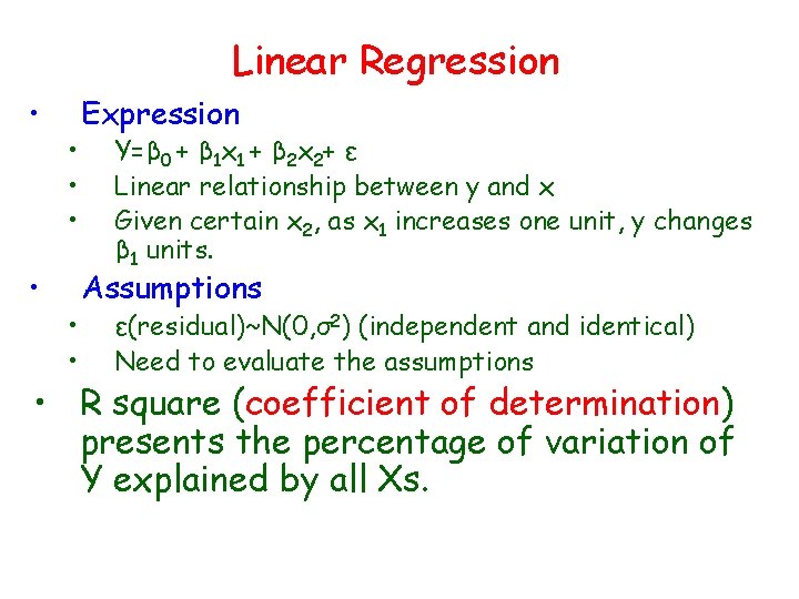
Linear Regression • • Expression Y=β 0 + β 1 x 1 + β 2 x 2+ ε Linear relationship between y and x Given certain x 2, as x 1 increases one unit, y changes β 1 units. Assumptions ε(residual)~N(0, σ2) (independent and identical) Need to evaluate the assumptions • R square (coefficient of determination) presents the percentage of variation of Y explained by all Xs.

Data Set • Lead exposure data • Effects of lead exposure on neurological and psychological function in children • Neurological endpoint – Maxfwt: maximum finger wrist tapping • Independent variables: Group (exposed to lead or not), age, sex, area

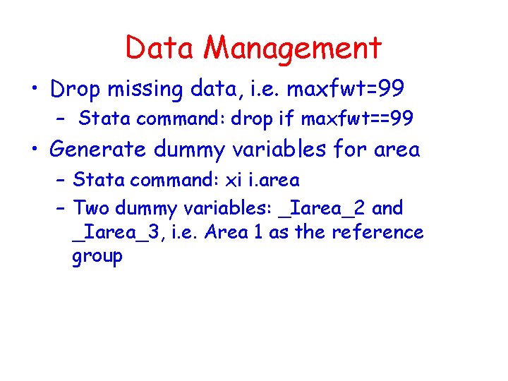
Data Management • Drop missing data, i. e. maxfwt=99 – Stata command: drop if maxfwt==99 • Generate dummy variables for area – Stata command: xi i. area – Two dummy variables: _Iarea_2 and _Iarea_3, i. e. Area 1 as the reference group

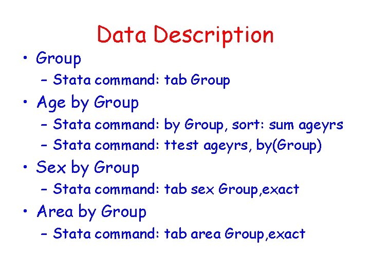
• Group Data Description – Stata command: tab Group • Age by Group – Stata command: by Group, sort: sum ageyrs – Stata command: ttest ageyrs, by(Group) • Sex by Group – Stata command: tab sex Group, exact • Area by Group – Stata command: tab area Group, exact

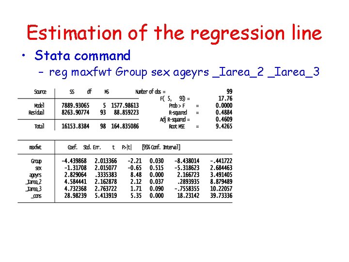
Estimation of the regression line • Stata command – reg maxfwt Group sex ageyrs _Iarea_2 _Iarea_3

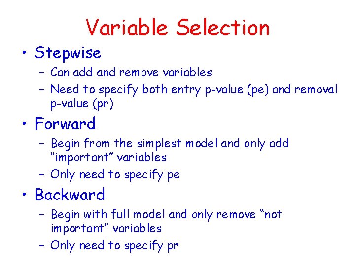
Variable Selection • Stepwise – Can add and remove variables – Need to specify both entry p-value (pe) and removal p-value (pr) • Forward – Begin from the simplest model and only add “important” variables – Only need to specify pe • Backward – Begin with full model and only remove “not important” variables – Only need to specify pr

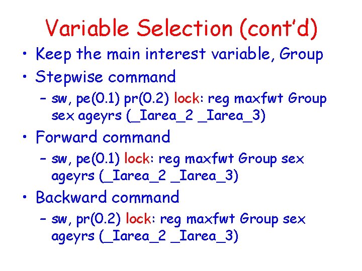
Variable Selection (cont’d) • Keep the main interest variable, Group • Stepwise command – sw, pe(0. 1) pr(0. 2) lock: reg maxfwt Group sex ageyrs (_Iarea_2 _Iarea_3) • Forward command – sw, pe(0. 1) lock: reg maxfwt Group sex ageyrs (_Iarea_2 _Iarea_3) • Backward command – sw, pr(0. 2) lock: reg maxfwt Group sex ageyrs (_Iarea_2 _Iarea_3)

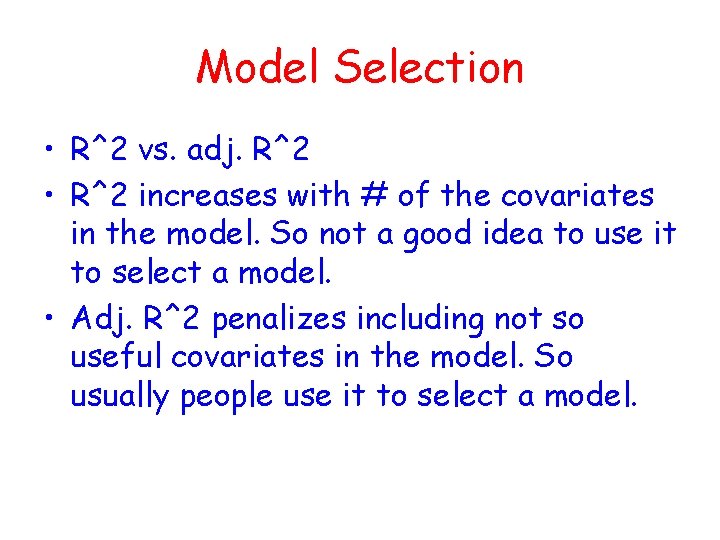
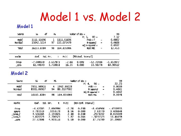
Model Selection • R^2 vs. adj. R^2 • R^2 increases with # of the covariates in the model. So not a good idea to use it to select a model. • Adj. R^2 penalizes including not so useful covariates in the model. So usually people use it to select a model.

Model 1 Model 2 Model 1 vs. Model 2

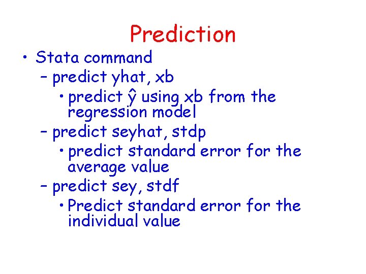
Prediction • Stata command – predict yhat, xb • predict ŷ using xb from the regression model – predict seyhat, stdp • predict standard error for the average value – predict sey, stdf • Predict standard error for the individual value

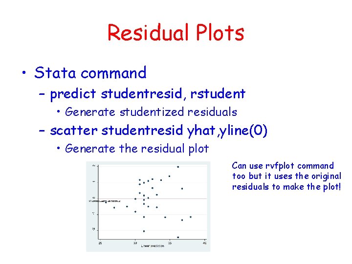
Residual Plots • Stata command – predict studentresid, rstudent • Generate studentized residuals – scatter studentresid yhat, yline(0) • Generate the residual plot Can use rvfplot command too but it uses the original residuals to make the plot!

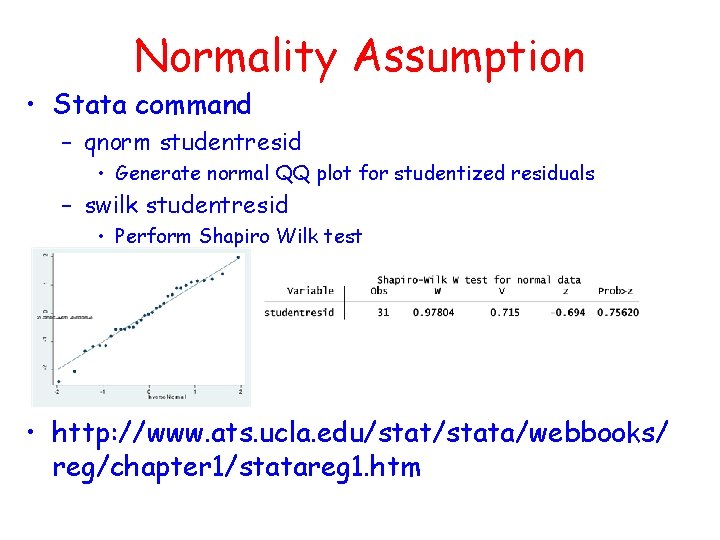
Normality Assumption • Stata command – qnorm studentresid • Generate normal QQ plot for studentized residuals – swilk studentresid • Perform Shapiro Wilk test • http: //www. ats. ucla. edu/stata/webbooks/ reg/chapter 1/statareg 1. htm