Stata Workshop 1 ChiuHsieh Paul Hsu Associate Professor

Stata Workshop #1 Chiu-Hsieh (Paul) Hsu Associate Professor College of Public Health pchhsu@email. arizona. edu

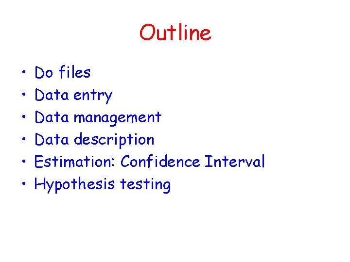
Outline • • • Do files Data entry Data management Data description Estimation: Confidence Interval Hypothesis testing

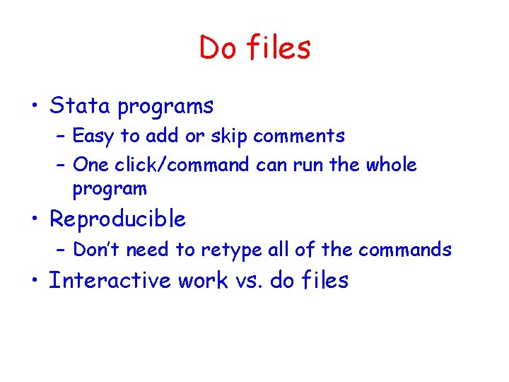
Do files • Stata programs – Easy to add or skip comments – One click/command can run the whole program • Reproducible – Don’t need to retype all of the commands • Interactive work vs. do files

Data Entry

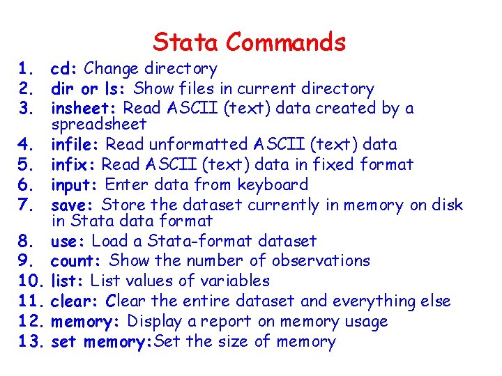
Stata Commands 1. cd: Change directory 2. dir or ls: Show files in current directory 3. insheet: Read ASCII (text) data created by a spreadsheet 4. infile: Read unformatted ASCII (text) data 5. infix: Read ASCII (text) data in fixed format 6. input: Enter data from keyboard 7. save: Store the dataset currently in memory on disk in Stata data format 8. use: Load a Stata-format dataset 9. count: Show the number of observations 10. list: List values of variables 11. clear: Clear the entire dataset and everything else 12. memory: Display a report on memory usage 13. set memory: Set the size of memory

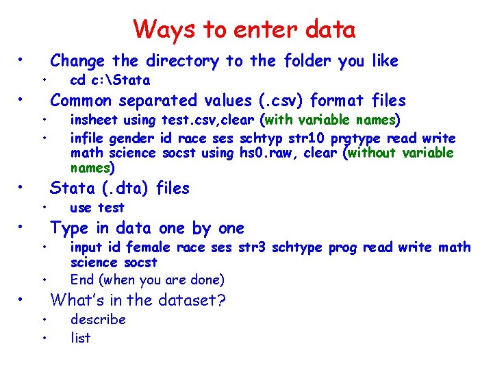
Ways to enter data • • • • Change the directory to the folder you like cd c: Stata Common separated values (. csv) format files insheet using test. csv, clear (with variable names) infile gender id race ses schtyp str 10 prgtype read write math science socst using hs 0. raw, clear (without variable names) Stata (. dta) files use test Type in data one by one input id female race ses str 3 schtype prog read write math science socst End (when you are done) What’s in the dataset? describe list

Data Management

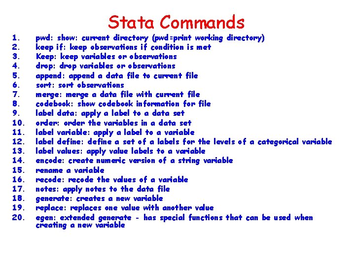
1. 2. 3. 4. 5. 6. 7. 8. 9. 10. 11. 12. 13. 14. 15. 16. 17. 18. 19. 20. Stata Commands pwd: show: current directory (pwd=print working directory) keep if: keep observations if condition is met Keep: keep variables or observations drop: drop variables or observations append: append a data file to current file sort: sort observations merge: merge a data file with current file codebook: show codebook information for file label data: apply a label to a data set order: order the variables in a data set label variable: apply a label to a variable label define: define a set of a labels for the levels of a categorical variable label values: apply value labels to a variable encode: create numeric version of a string variable rename a variable recode: recode the values of a variable notes: apply notes to the data file generate: creates a new variable replace: replaces one value with another value egen: extended generate - has special functions that can be used when creating a new variable

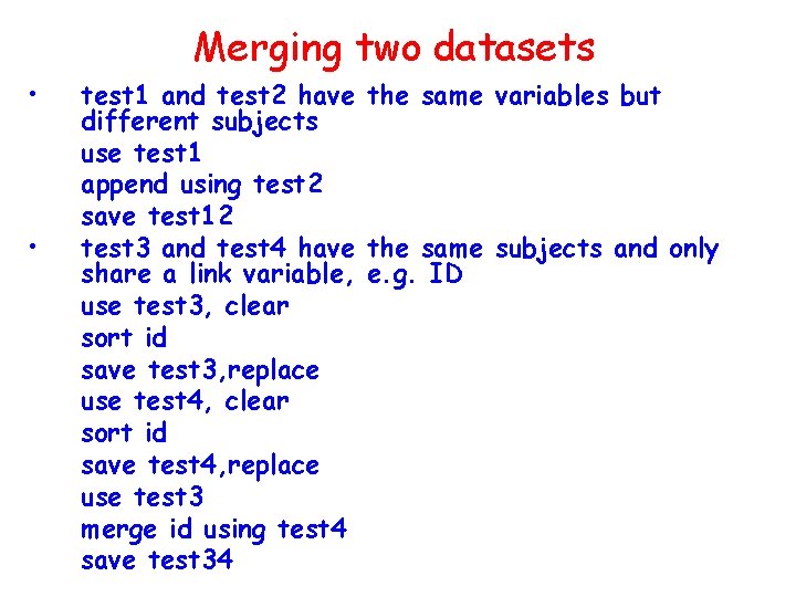
Merging two datasets • • test 1 and test 2 have the same variables but different subjects use test 1 append using test 2 save test 12 test 3 and test 4 have the same subjects and only share a link variable, e. g. ID use test 3, clear sort id save test 3, replace use test 4, clear sort id save test 4, replace use test 3 merge id using test 4 save test 34

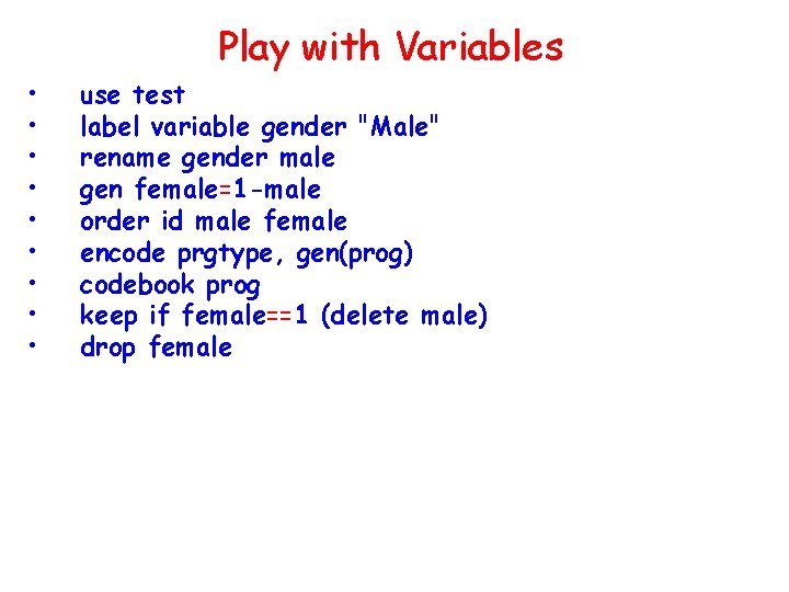
Play with Variables • • • use test label variable gender "Male" rename gender male gen female=1 -male order id male female encode prgtype, gen(prog) codebook prog keep if female==1 (delete male) drop female

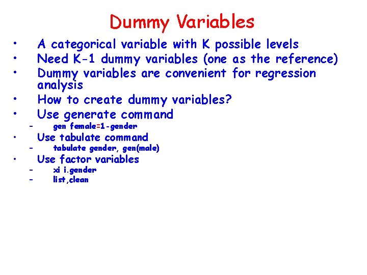
Dummy Variables • • – – A categorical variable with K possible levels Need K-1 dummy variables (one as the reference) Dummy variables are convenient for regression analysis How to create dummy variables? Use generate command gen female=1 -gender Use tabulate command tabulate gender, gen(male) Use factor variables xi i. gender list, clean

Data Description

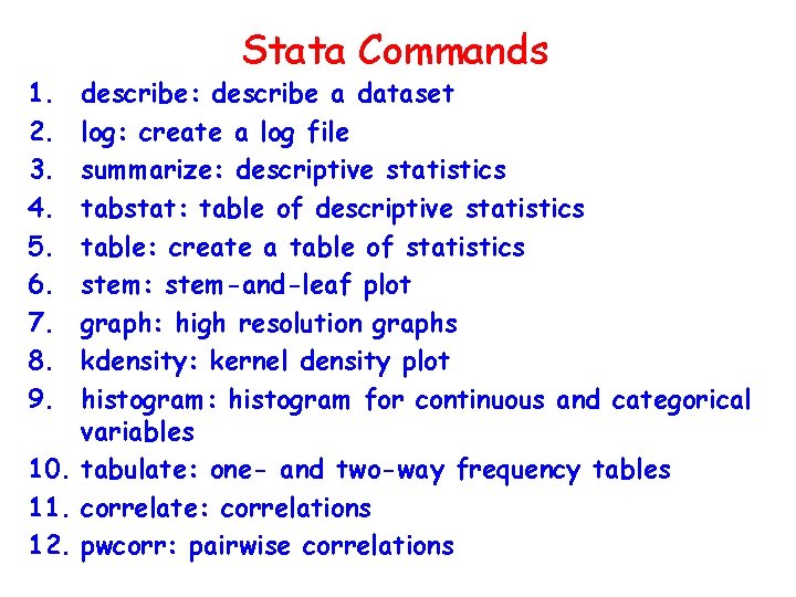
1. 2. 3. 4. 5. 6. 7. 8. 9. Stata Commands describe: describe a dataset log: create a log file summarize: descriptive statistics tabstat: table of descriptive statistics table: create a table of statistics stem: stem-and-leaf plot graph: high resolution graphs kdensity: kernel density plot histogram: histogram for continuous and categorical variables 10. tabulate: one- and two-way frequency tables 11. correlate: correlations 12. pwcorr: pairwise correlations

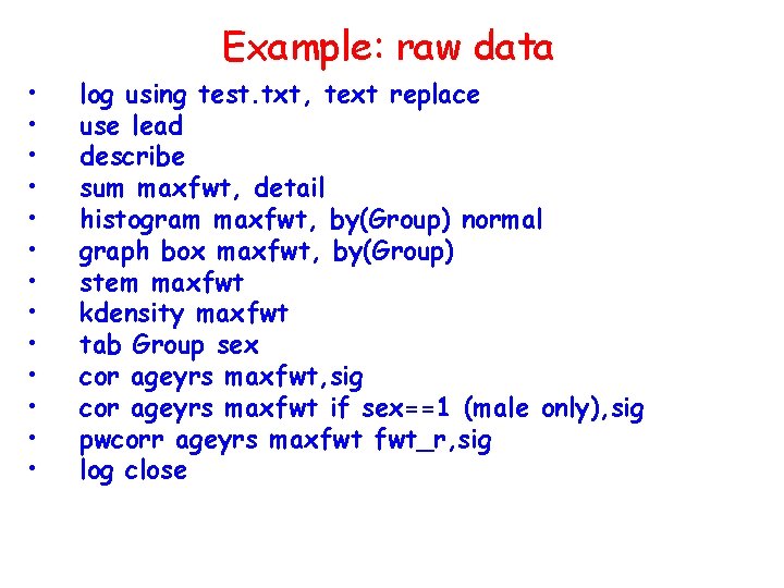
Example: raw data • • • • log using test. txt, text replace use lead describe sum maxfwt, detail histogram maxfwt, by(Group) normal graph box maxfwt, by(Group) stem maxfwt kdensity maxfwt tab Group sex cor ageyrs maxfwt, sig cor ageyrs maxfwt if sex==1 (male only), sig pwcorr ageyrs maxfwt fwt_r, sig log close

Example: grouped data • • use group (a grouped dataset) sum age [fweight=freq], detail hist age [fweight=freq] Pretty much the same as raw data. Just need to specify the weight.

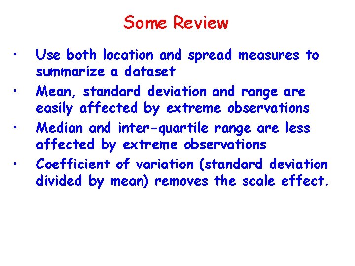
Some Review • • Use both location and spread measures to summarize a dataset Mean, standard deviation and range are easily affected by extreme observations Median and inter-quartile range are less affected by extreme observations Coefficient of variation (standard deviation divided by mean) removes the scale effect.

Estimation

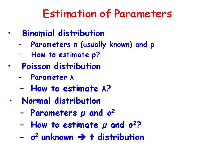
Estimation of Parameters • Binomial distribution – – • Parameters n (usually known) and p How to estimate p? Poisson distribution – Parameter λ – How to estimate λ? • Normal distribution – Parameters µ and σ2 – How to estimate µ and σ2? – σ2 unknown t distribution

Stata Commands • Raw data – ci [varlist] [if] [in] [weight] [, options] • • confidence intervals for mean, proportion (b) and count (p) Summarry statistics – cii #obs #mean #sd [, ciin_option] • – Normal cii #obs #succ [, ciib_options] • Binomial

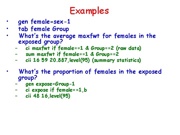
Examples • • • – – – gen female=sex-1 tab female Group What’s the average maxfwt for females in the exposed group? ci maxfwt if female==1 & Group==2 (raw data) sum maxfwt if female==1 & Group==2 cii 16 59 20. 887, level(95) (summary statistics) What’s the proportion of females in the exposed group? gen expose=Group-1 ci expose if female==1, b cii 48 16, level(95)

Hypothesis Testing

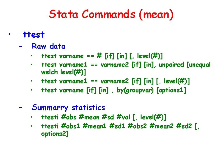
Stata Commands (mean) • ttest – Raw data • • – ttest varname == # [if] [in] [, level(#)] ttest varname 1 == varname 2 [if] [in], unpaired [unequal welch level(#)] ttest varname 1 == varname 2 [if] [in] [, level(#)] ttest varname [if] [in] , by(groupvar) [options 1] Summarry statistics • • ttesti #obs #mean #sd #val [, level(#)] ttesti #obs 1 #mean 1 #sd 1 #obs 2 #mean 2 #sd 2 [, options 2]

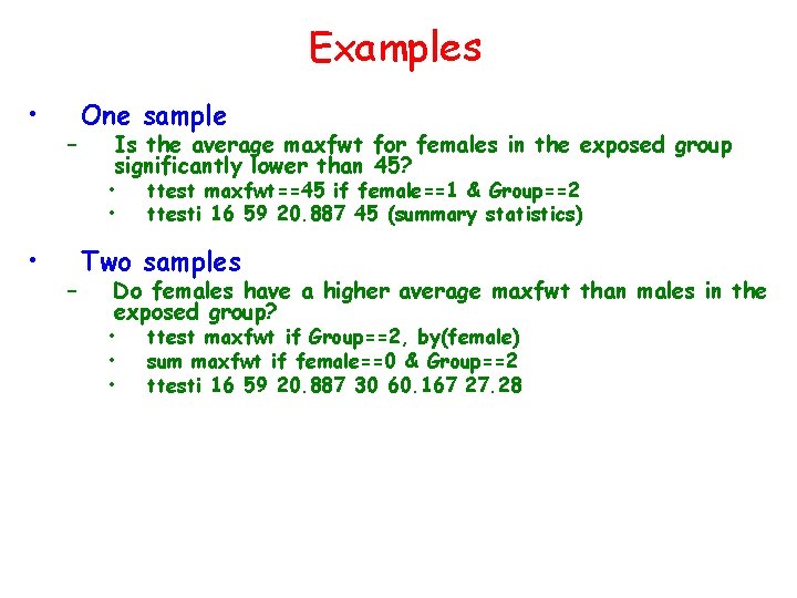
Examples • – One sample Is the average maxfwt for females in the exposed group significantly lower than 45? • • • – ttest maxfwt==45 if female==1 & Group==2 ttesti 16 59 20. 887 45 (summary statistics) Two samples Do females have a higher average maxfwt than males in the exposed group? • • • ttest maxfwt if Group==2, by(female) sum maxfwt if female==0 & Group==2 ttesti 16 59 20. 887 30 60. 167 27. 28

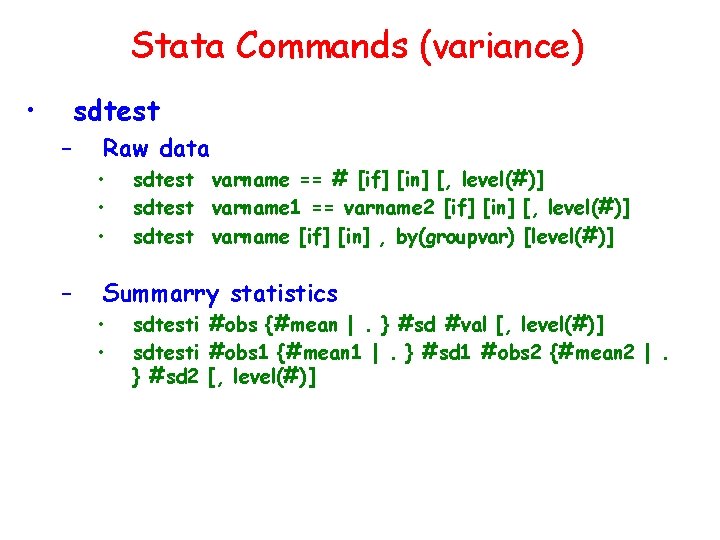
Stata Commands (variance) • sdtest – Raw data • • • – sdtest varname == # [if] [in] [, level(#)] sdtest varname 1 == varname 2 [if] [in] [, level(#)] sdtest varname [if] [in] , by(groupvar) [level(#)] Summarry statistics • • sdtesti #obs {#mean |. } #sd #val [, level(#)] sdtesti #obs 1 {#mean 1 |. } #sd 1 #obs 2 {#mean 2 |. } #sd 2 [, level(#)]

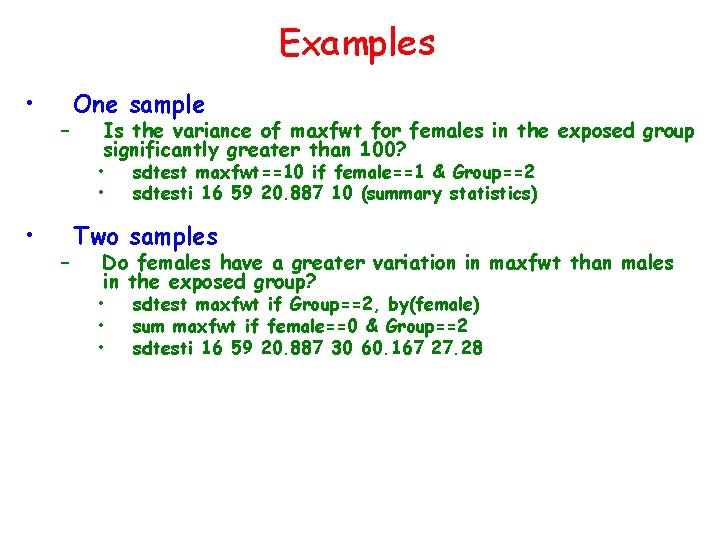
Examples • – One sample Is the variance of maxfwt for females in the exposed group significantly greater than 100? • • • – sdtest maxfwt==10 if female==1 & Group==2 sdtesti 16 59 20. 887 10 (summary statistics) Two samples Do females have a greater variation in maxfwt than males in the exposed group? • • • sdtest maxfwt if Group==2, by(female) sum maxfwt if female==0 & Group==2 sdtesti 16 59 20. 887 30 60. 167 27. 28

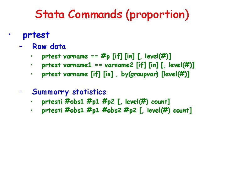
Stata Commands (proportion) • prtest – Raw data • • • – prtest varname == #p [if] [in] [, level(#)] prtest varname 1 == varname 2 [if] [in] [, level(#)] prtest varname [if] [in] , by(groupvar) [level(#)] Summarry statistics • • prtesti #obs 1 #p 2 [, level(#) count] prtesti #obs 1 #p 1 #obs 2 #p 2 [, level(#) count]

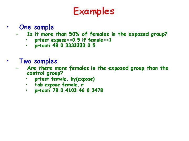
Examples • • – – One sample Is it more than 50% of females in the exposed group? • • prtest expose==0. 5 if female==1 prtesti 48 0. 3333333 0. 5 Two samples Are there more females in the exposed group than the control group? • • • prtest female, by(expose) tab expose female, r prtesti 78 0. 4103 46 0. 3478

Power and Sample Size

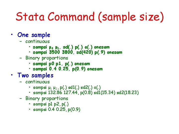
Stata Command (sample size) • One sample – continuous • sampsi μ 0 μ 1, sd(. ) p(. ) a(. ) onesam • sampsi 3500 3800, sd(420) p(. 9) onesam – Binary proportions • sampsi p 0 p 1, p(. ) onesam • sampsi 0. 4 0. 25, p(0. 9) onesam • Two samples – continuous • sampsi μ 1 μ 2, p(. ) sd 1(. ) sd 2(. ) a(. ) • sampsi 132. 86 127. 44, p(0. 8) sd 1(15. 34) sd 2(18. 23) – Binary proportions • sampsi p 1 p 2, p(. ) • sampsi 0. 4 0. 25, p(0. 9)

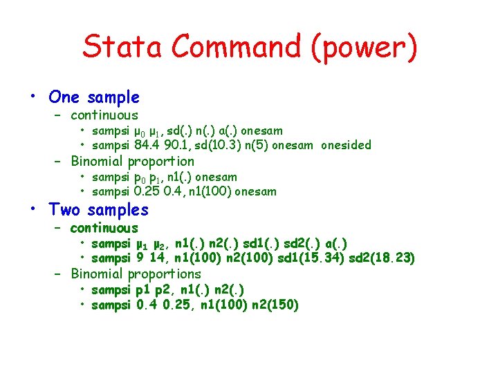
Stata Command (power) • One sample – continuous • sampsi μ 0 μ 1, sd(. ) n(. ) a(. ) onesam • sampsi 84. 4 90. 1, sd(10. 3) n(5) onesam onesided – Binomial proportion • sampsi p 0 p 1, n 1(. ) onesam • sampsi 0. 25 0. 4, n 1(100) onesam • Two samples – continuous • sampsi μ 1 μ 2, n 1(. ) n 2(. ) sd 1(. ) sd 2(. ) a(. ) • sampsi 9 14, n 1(100) n 2(100) sd 1(15. 34) sd 2(18. 23) – Binomial proportions • sampsi p 1 p 2, n 1(. ) n 2(. ) • sampsi 0. 4 0. 25, n 1(100) n 2(150)

Useful links • http: //www. ats. ucla. edu/stata/ • Once the D 2 L site is created, all of the handouts and related materials will be posted on the D 2 L site.