Stata Linear Regression 2 h Hein Stigum Presentation

Stata: Linear Regression 2 h Hein Stigum Presentation, data and programs at: http: //folk. uio. no/heins/ courses Dec-20 H. S. 1

DAG, Table 1 and Table 2 INTRODUCTION Dec-20 H. S. 2

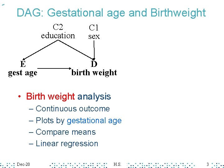
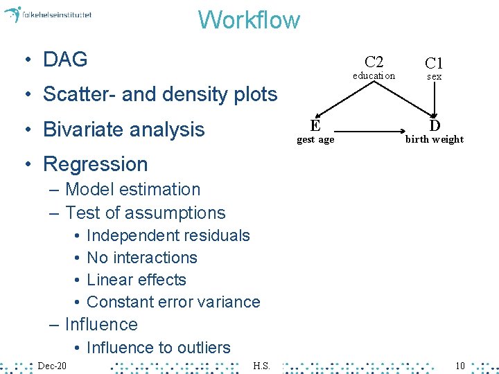
DAG: Gestational age and Birthweight C 2 education E gest age C 1 sex D birth weight • Birth weight analysis – Continuous outcome – Plots by gestational age – Compare means – Linear regression Dec-20 H. S. 3

Agenda • Purpose • Workflow • Syntax • Testing assumptions • Influence Dec-20 H. S. 4

BACKGROUND Dec-20 H. S. 5

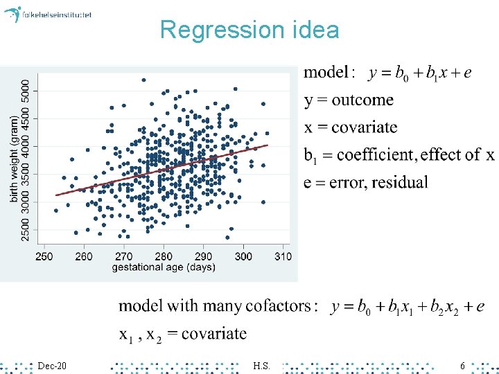
Regression idea Dec-20 H. S. 6

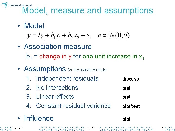
Model, measure and assumptions • Model • Association measure b 1 = change in y for one unit increase in x 1 • Assumptions for the standard model 1. 2. 3. 4. Independent residuals No interactions Linear effects Constant residual variance • Influence Dec-20 discuss test plot/test plot H. S. 7

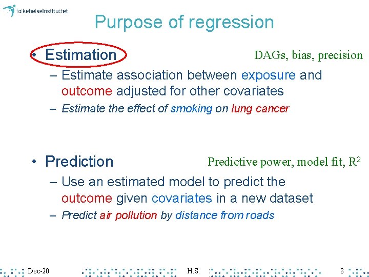
Purpose of regression • Estimation DAGs, bias, precision – Estimate association between exposure and outcome adjusted for other covariates – Estimate the effect of smoking on lung cancer • Prediction Predictive power, model fit, R 2 – Use an estimated model to predict the outcome given covariates in a new dataset – Predict air pollution by distance from roads Dec-20 H. S. 8

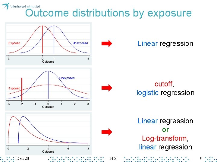
Outcome distributions by exposure Linear regression cutoff, logistic regression Linear regression or Log-transform, linear regression Dec-20 H. S. 9

Workflow • DAG C 2 education • Scatter- and density plots E • Bivariate analysis gest age C 1 sex D birth weight • Regression – Model estimation – Test of assumptions • • Independent residuals No interactions Linear effects Constant error variance – Influence • Influence to outliers Dec-20 H. S. 10

Syntax: “ 3 Linear Regression. do” “Analysis” Dec-20 H. S. 11

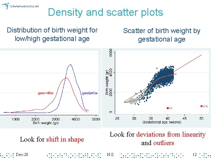
Density and scatter plots Distribution of birth weight for low/high gestational age Look for shift in shape Dec-20 Scatter of birth weight by gestational age Look for deviations from linearity and outliers H. S. 12

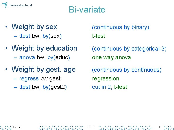
Bi-variate • Weight by sex – ttest bw, by(sex) • Weight by education – anova bw, by(educ) • Weight by gest. age – regress bw gest – ttest bw, by(gest 2) Dec-20 (continuous by binary) t-test (continuous by categorical-3) one way anova (continuous by continuous) regression cut in 2, t-test H. S. 13

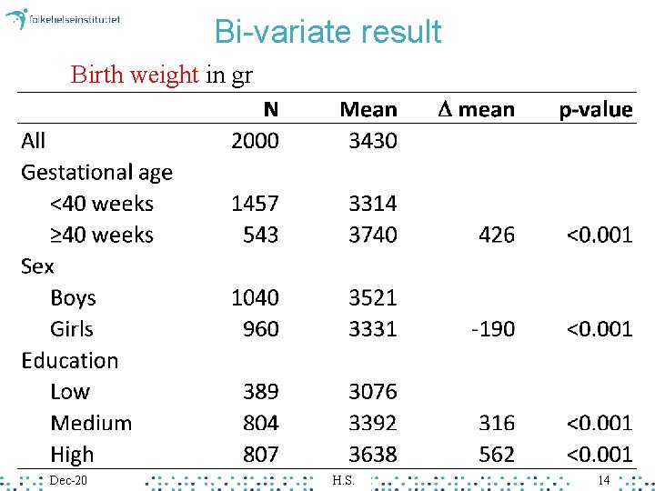
Bi-variate result Birth weight in gr Dec-20 H. S. 14

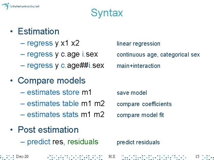
Syntax • Estimation – regress y x 1 x 2 – regress y c. age i. sex – regress y c. age##i. sex linear regression continuous age, categorical sex main+interaction • Compare models – estimates store m 1 – estimates table m 1 m 2 – estimates stats m 1 m 2 save model compare coefficients compare model fit • Post estimation – predict res, residuals Dec-20 predict residuals H. S. 15

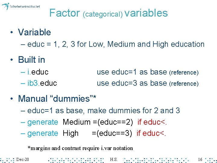
Factor (categorical) variables • Variable – educ = 1, 2, 3 for Low, Medium and High education • Built in – i. educ – ib 3. educ use educ=1 as base (reference) use educ=3 as base (reference) • Manual “dummies”* – educ=1 as base, make dummies for 2 and 3 – generate Medium =(educ==2) if educ<. – generate High =(educ==3) if educ<. *margins and contrast require i. var notation Dec-20 H. S. 16

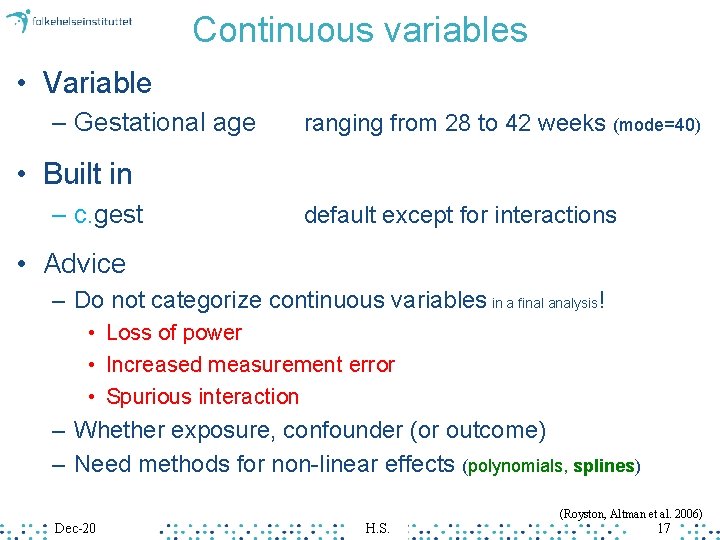
Continuous variables • Variable – Gestational age ranging from 28 to 42 weeks (mode=40) • Built in – c. gest default except for interactions • Advice – Do not categorize continuous variables in a final analysis! • Loss of power • Increased measurement error • Spurious interaction – Whether exposure, confounder (or outcome) – Need methods for non-linear effects (polynomials, splines) (Royston, Altman et al. 2006) Dec-20 H. S. 17

Syntax “Regression analysis” Dec-20 H. S. 18

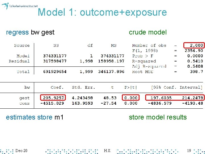
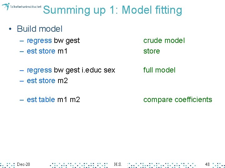
Model 1: outcome+exposure regress bw gest crude model estimates store m 1 store model results Dec-20 H. S. 19

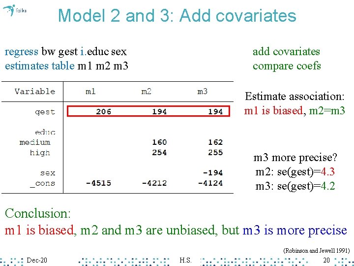
Model 2 and 3: Add covariates regress bw gest i. educ sex estimates table m 1 m 2 m 3 add covariates compare coefs Estimate association: m 1 is biased, m 2=m 3 more precise? m 2: se(gest)=4. 3 m 3: se(gest)=4. 2 Conclusion: m 1 is biased, m 2 and m 3 are unbiased, but m 3 is more precise (Robinson and Jewell 1991) Dec-20 H. S. 20

Measures of influence INFLUENCE WOULD NORMALLY HANDLE ASSUMPTIONS FIRST Dec-20 H. S. 21

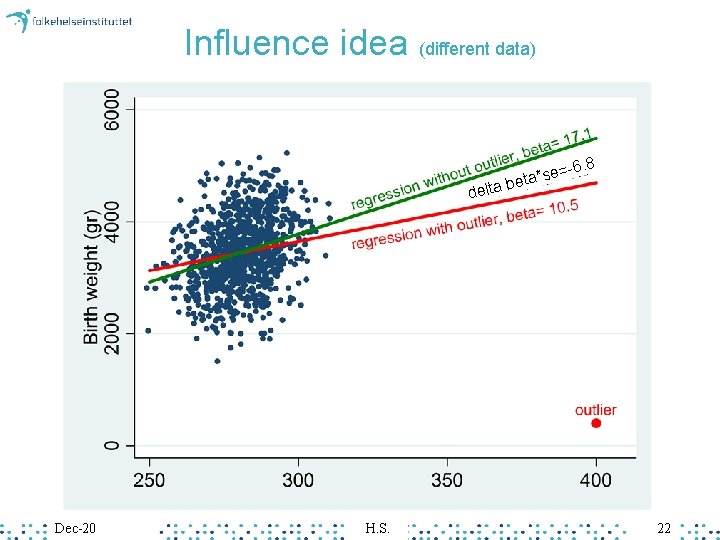
Influence idea (different data) 6. 8 delta Dec-20 H. S. se=* a t e b 22

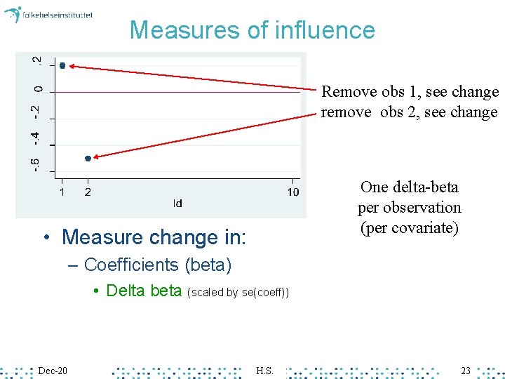
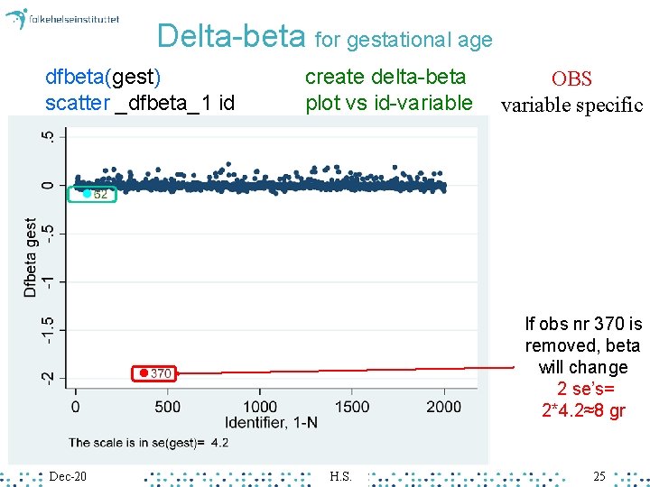
Measures of influence Remove obs 1, see change remove obs 2, see change One delta-beta per observation (per covariate) • Measure change in: – Coefficients (beta) • Delta beta (scaled by se(coeff)) Dec-20 H. S. 23

Syntax: “Influence of outliers” Dec-20 H. S. 24

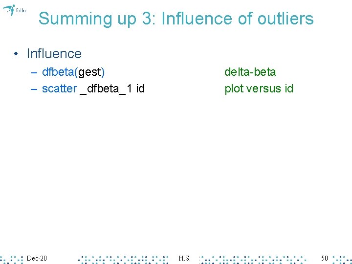
Delta-beta for gestational age dfbeta(gest) scatter _dfbeta_1 id create delta-beta plot vs id-variable OBS variable specific If obs nr 370 is removed, beta will change 2 se’s= 2*4. 2≈8 gr Dec-20 H. S. 25

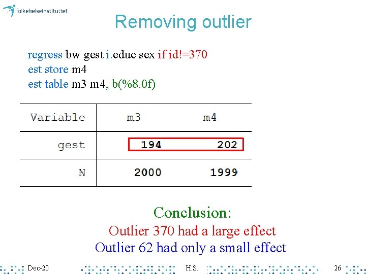
Removing outlier regress bw gest i. educ sex if id!=370 est store m 4 est table m 3 m 4, b(%8. 0 f) Conclusion: Outlier 370 had a large effect Outlier 62 had only a small effect Dec-20 H. S. 26

ASSUMPTIONS Dec-20 H. S. 27

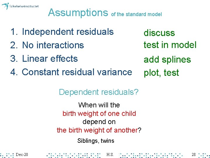
Assumptions of the standard model 1. 2. 3. 4. Independent residuals No interactions Linear effects Constant residual variance discuss test in model add splines plot, test Dependent residuals? When will the birth weight of one child depend on the birth weight of another? Siblings, twins Dec-20 H. S. 28

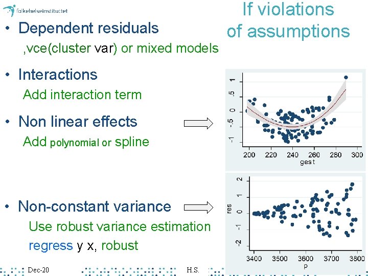
• Dependent residuals , vce(cluster var) or mixed models If violations of assumptions • Interactions Add interaction term • Non linear effects Add polynomial or spline • Non-constant variance Use robust variance estimation regress y x, robust Dec-20 H. S. 29

INTERACTION ONLY LINEAR EFFECTS Dec-20 H. S. 30

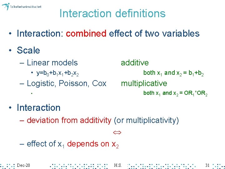
Interaction definitions • Interaction: combined effect of two variables • Scale – Linear models additive • y=b 0+b 1 x 1+b 2 x 2 – Logistic, Poisson, Cox both x 1 and x 2 = b 1+b 2 multiplicative both x 1 and x 2 = OR 1*OR 2 • • Interaction – deviation from additivity (or multiplicativity) – effect of x 1 depends on x 2 Dec-20 H. S. 31

Syntax “Interaction” Dec-20 H. S. 32

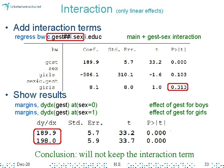
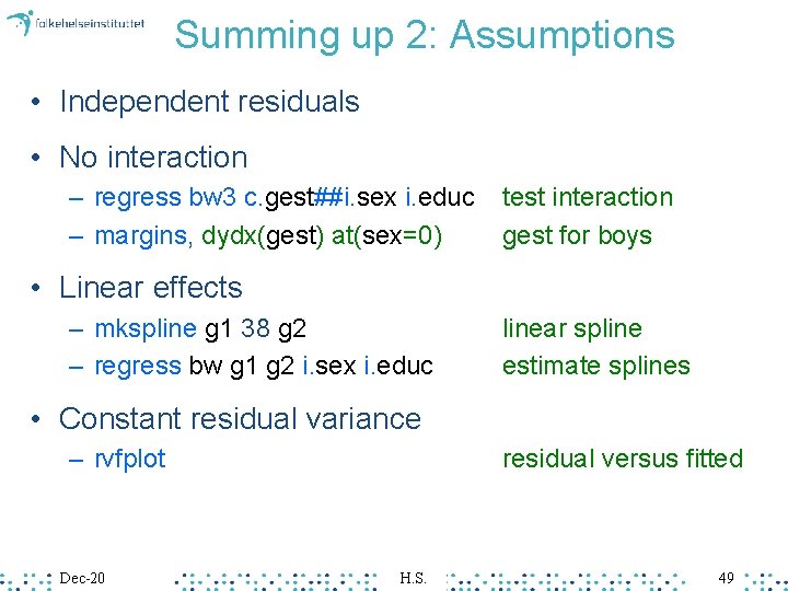
Interaction (only linear effects) • Add interaction terms regress bw c. gest##i. sex i. educ main + gest-sex interaction • Show results margins, dydx(gest) at(sex=0) margins, dydx(gest) at(sex=1) effect of gest for boys effect of gest for girls Conclusion: will not keep the interaction term Dec-20 H. S. 33

NON-LINEAR EFFECTS Dec-20 H. S. 34

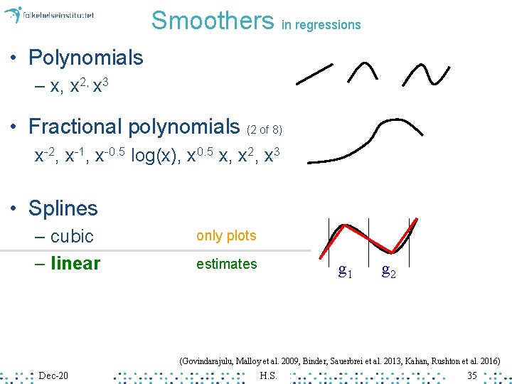
Smoothers in regressions • Polynomials – x, x 2, x 3 • Fractional polynomials (2 of 8) x-2, x-1, x-0. 5 log(x), x 0. 5 x, x 2, x 3 • Splines – cubic – linear only plots estimates g 1 g 2 (Govindarajulu, Malloy et al. 2009, Binder, Sauerbrei et al. 2013, Kahan, Rushton et al. 2016) Dec-20 H. S. 35

Syntax “Linear effect” Dec-20 H. S. 36

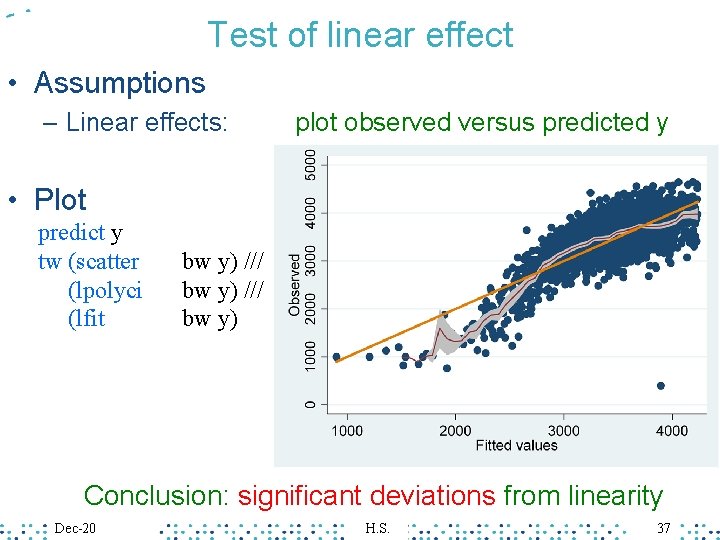
Test of linear effect • Assumptions – Linear effects: plot observed versus predicted y • Plot predict y tw (scatter (lpolyci (lfit bw y) /// bw y) Conclusion: significant deviations from linearity Dec-20 H. S. 37

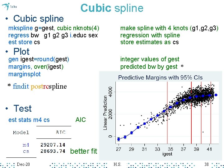
• Cubic spline mkspline g=gest, cubic nknots(4) regress bw g 1 g 2 g 3 i. educ sex est store cs • Plot gen igest=round(gest) margins, over(igest) marginsplot make spline with 4 knots (g 1, g 2, g 3) regression with spline store estimates as cs integer values of gest predicted bw by gest * plot * findit postrcspline • Test stats m 4 cs AIC better fit Dec-20 H. S. 38

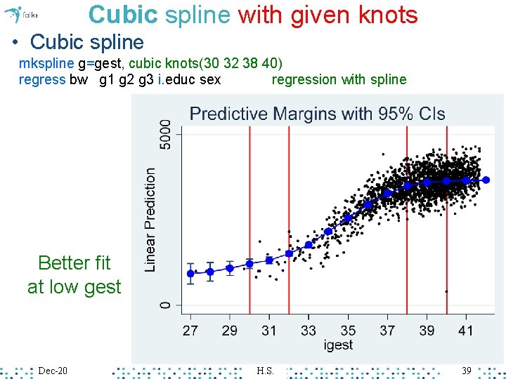
Cubic spline with given knots • Cubic spline mkspline g=gest, cubic knots(30 32 38 40) regress bw g 1 g 2 g 3 i. educ sex regression with spline Better fit at low gest Dec-20 H. S. 39

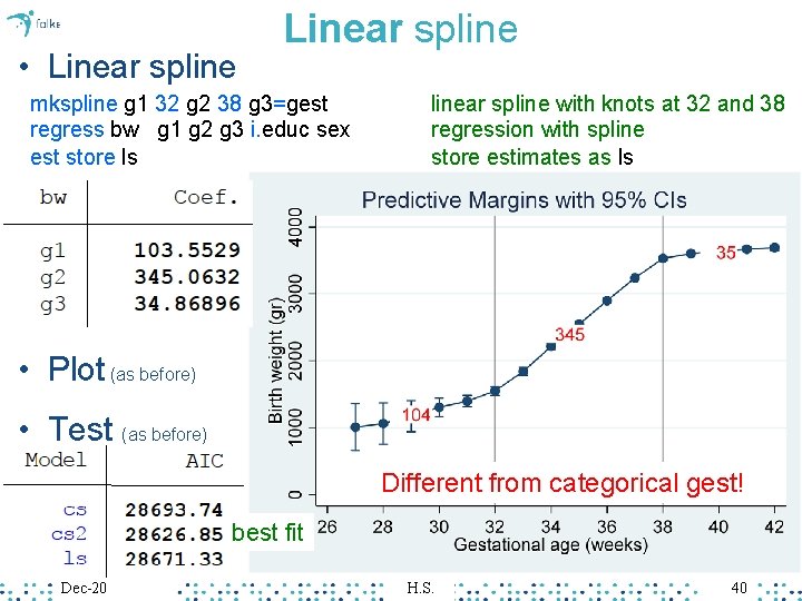
• Linear spline mkspline g 1 32 g 2 38 g 3=gest regress bw g 1 g 2 g 3 i. educ sex est store ls linear spline with knots at 32 and 38 regression with spline store estimates as ls • Plot (as before) • Test (as before) Different from categorical gest! best fit Dec-20 H. S. 40

Summing up: non-linear effects • Capture non-linearities in continuous variable – Categorize, lose precision – Fractional polynomials or splines • Continuous exposure – Replace by cubic spline: good fit, only plot – Replace by linear spline: good fit, estimates • Continuous confounder – Keep linear Dec-20 H. S. 41

CONSTANT RESIDUAL VARIANCE Dec-20 H. S. 42

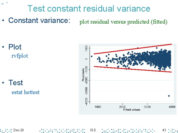
Test constant residual variance • Constant variance: plot residual versus predicted (fitted) • Plot rvfplot • Test estat hettest Dec-20 H. S. 43

Syntax : “Constant residual variance” Dec-20 H. S. 44

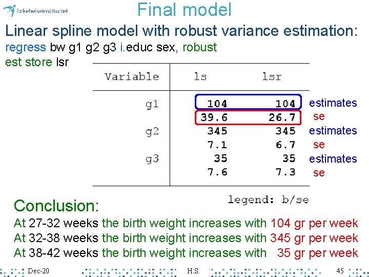
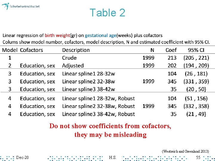
Final model Linear spline model with robust variance estimation: regress bw g 1 g 2 g 3 i. educ sex, robust est store lsr estimates se Conclusion: At 27 -32 weeks the birth weight increases with 104 gr per week At 32 -38 weeks the birth weight increases with 345 gr per week At 38 -42 weeks the birth weight increases with 35 gr per week Dec-20 H. S. 45

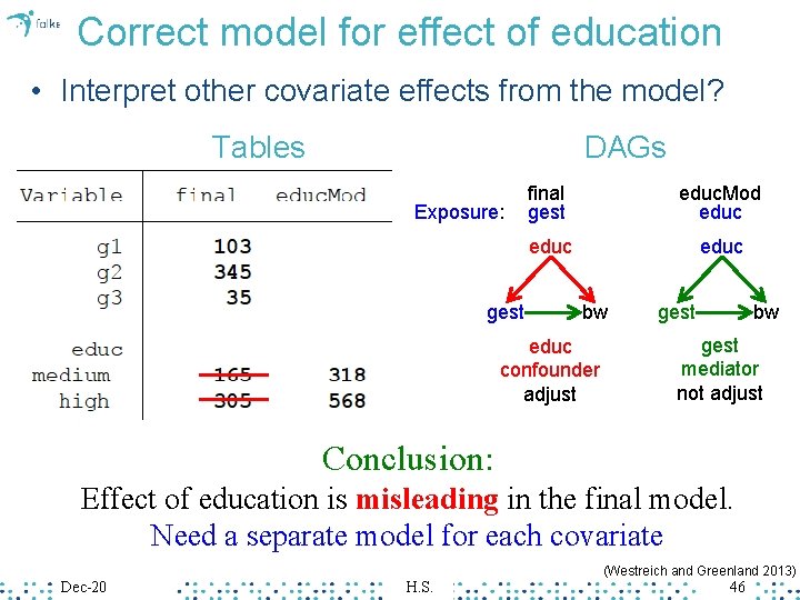
Correct model for effect of education • Interpret other covariate effects from the model? Tables DAGs Exposure: gest final gest educ. Mod educ bw educ confounder adjust gest bw gest mediator not adjust Conclusion: Effect of education is misleading in the final model. Need a separate model for each covariate (Westreich and Greenland 2013) Dec-20 H. S. 46

Help • Linear regression – help regress • syntax and options – help regress postestimation • • • dfbeta estat hettest rvfplot predict margins – help factor variables • factor variables and interactions Dec-20 H. S. 47

Summing up 1: Model fitting • Build model – regress bw gest – est store m 1 crude model store – regress bw gest i. educ sex – est store m 2 full model – est table m 1 m 2 compare coefficients Dec-20 H. S. 48

Summing up 2: Assumptions • Independent residuals • No interaction – regress bw 3 c. gest##i. sex i. educ – margins, dydx(gest) at(sex=0) test interaction gest for boys • Linear effects – mkspline g 1 38 g 2 – regress bw g 1 g 2 i. sex i. educ linear spline estimate splines • Constant residual variance – rvfplot Dec-20 residual versus fitted H. S. 49

Summing up 3: Influence of outliers • Influence – dfbeta(gest) – scatter _dfbeta_1 id Dec-20 delta-beta plot versus id H. S. 50

References • Westreich, D. and S. Greenland (2013). "The Table 2 Fallacy: Presenting and Interpreting Confounder and Modifier Coefficients. " American Journal of Epidemiology 177(4): 292 -298. • Robinson, L. D. and N. P. Jewell (1991). "Some Surprising Results About Covariate Adjustment in Logistic-Regression Models. " International Statistical Review 59(2): 227 -240. • Xing, C. and G. A. Xing (2010). "Adjusting for Covariates in Logistic Regression Models. " Genetic Epidemiology 34(8): 937 -937. • Royston, P. , D. G. Altman and W. Sauerbrei (2006). "Dichotomizing continuous predictors in multiple regression: a bad idea. " Stat Med 25(1): 127 -141. • Binder, H. , W. Sauerbrei and P. Royston (2013). "Comparison between splines and fractional polynomials for multivariable model building with continuous covariates: a simulation study with continuous response. " Stat Med 32(13): 2262 -2277. • Govindarajulu, U. S. , E. J. Malloy, B. Ganguli, D. Spiegelman and E. A. Eisen (2009). "The Comparison of Alternative Smoothing Methods for Fitting Non. Linear Exposure-Response Relationships with Cox Models in a Simulation Study. " International Journal of Biostatistics 5(1). • Kahan, B. C. , H. Rushton, T. P. Morris and R. M. Daniel (2016). "A comparison of methods to adjust for continuous covariates in the analysis of randomised trials. " BMC Med Res Methodol 16: 42. Dec-20 H. S. 51

EXTRA MATERIAL Dec-20 H. S. 52

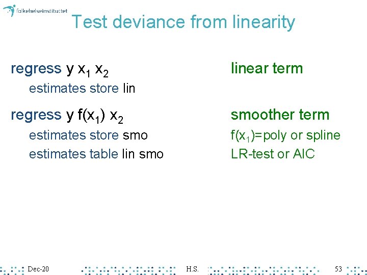
Test deviance from linearity regress y x 1 x 2 linear term estimates store lin regress y f(x 1) x 2 smoother term estimates store smo estimates table lin smo Dec-20 f(x 1)=poly or spline LR-test or AIC H. S. 53

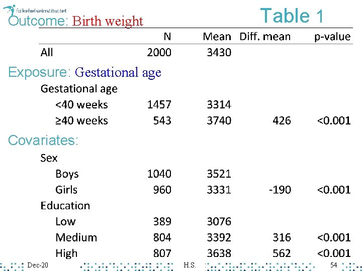
Table 1 Outcome: Birth weight Exposure: Gestational age Covariates: Dec-20 H. S. 54

Table 2 Do not show coefficients from cofactors, they may be misleading (Westreich and Greenland 2013) Dec-20 H. S. 55