STAT 515 Statistical Methods I Lecture 4 September

STAT 515 Statistical Methods I Lecture 4 September 3, 2019 Originally prepared by Brian Habing Department of Statistics University of South Carolina Redistribution of these slides without permission is a violation of copyright law.

Outline for Today • Finishing Probability Part I – Sections 3. 1 -3. 9 • Starting Probability Part II – Discrete Random Variables – Sections 4. 1 -4. 4 and 4. 6 • Homework 3 is due Thursday the 3 rd 3. 70, 3. 124 c, 3. 179 b • No homework due Tuesday the 8 th 2

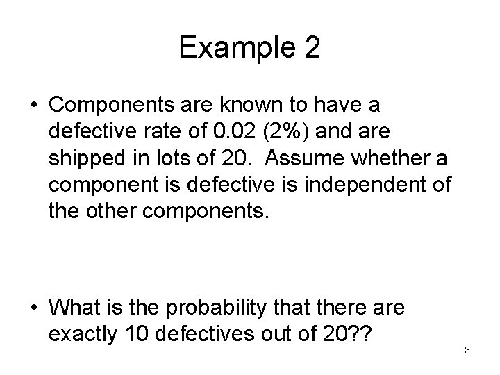
Example 2 • Components are known to have a defective rate of 0. 02 (2%) and are shipped in lots of 20. Assume whether a component is defective is independent of the other components. • What is the probability that there are exactly 10 defectives out of 20? ? 3

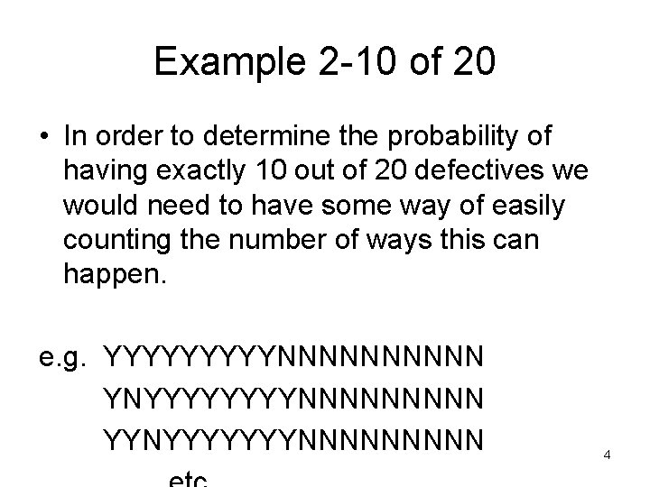
Example 2 -10 of 20 • In order to determine the probability of having exactly 10 out of 20 defectives we would need to have some way of easily counting the number of ways this can happen. e. g. YYYYYNNNNN YNYYYYNNNNN YYNYYYYYYYNNNNN 4

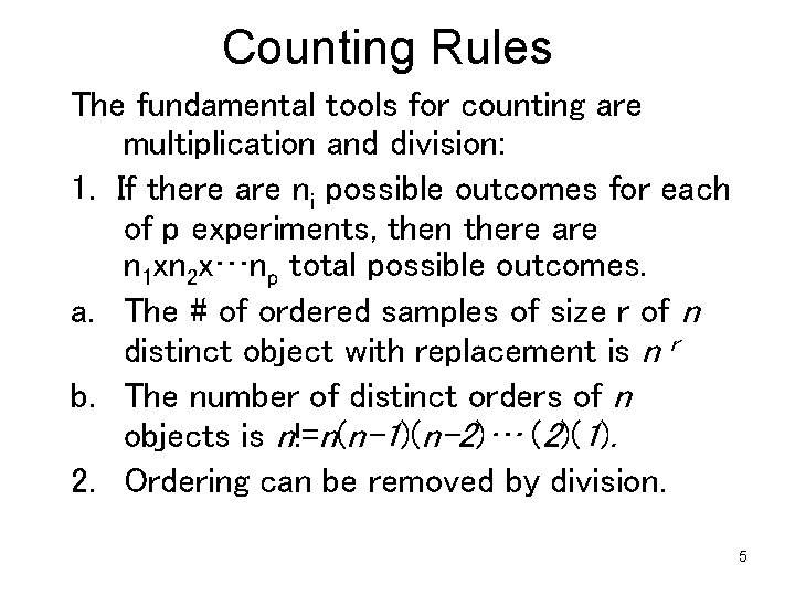
Counting Rules The fundamental tools for counting are multiplication and division: 1. If there are ni possible outcomes for each of p experiments, then there are n 1 xn 2 x…np total possible outcomes. a. The # of ordered samples of size r of n distinct object with replacement is n r b. The number of distinct orders of n objects is n!=n(n-1)(n-2)… (2)(1). 2. Ordering can be removed by division. 5

Sampling r objects Number of Samples of Size r Ordered With Replacement nr Unordered (n -1+r )! r ! (n -1)! Without Replacement n! (n –r )! permutation n! r !(n-r )! combination 6

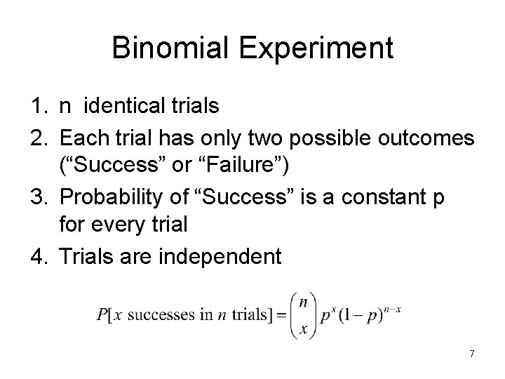
Binomial Experiment 1. n identical trials 2. Each trial has only two possible outcomes (“Success” or “Failure”) 3. Probability of “Success” is a constant p for every trial 4. Trials are independent 7

Why doesn’t this work for opinion polls? 8

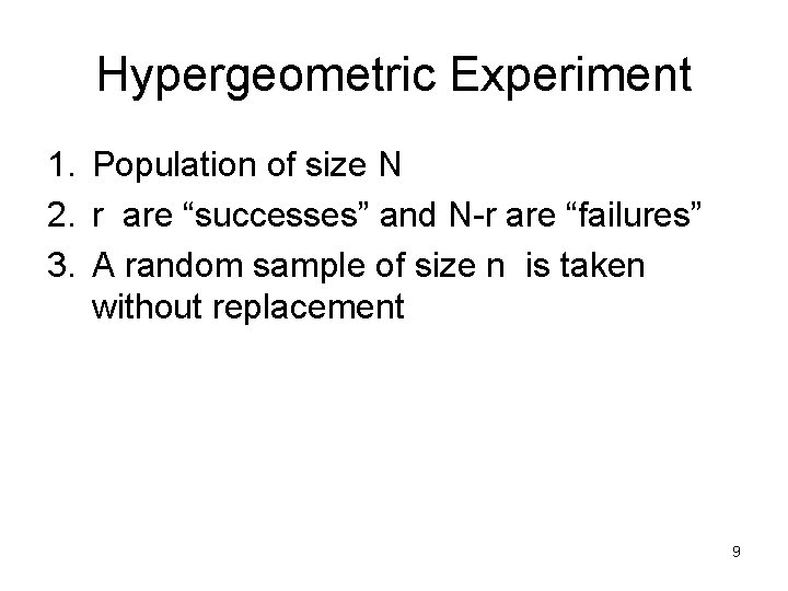
Hypergeometric Experiment 1. Population of size N 2. r are “successes” and N-r are “failures” 3. A random sample of size n is taken without replacement 9

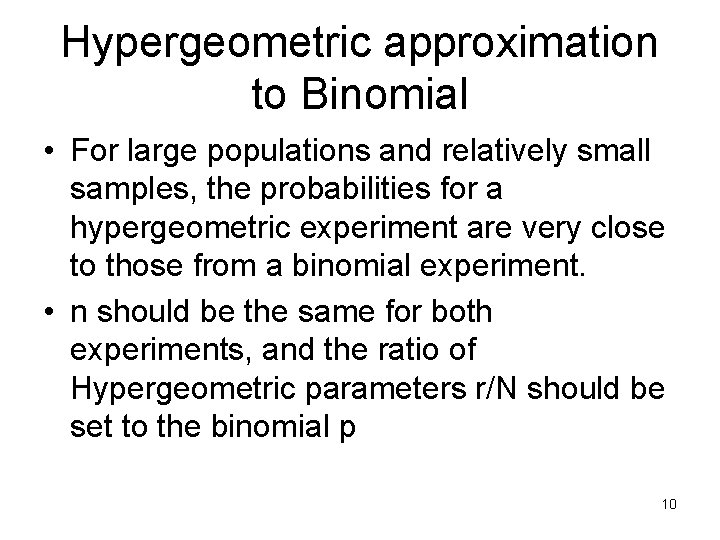
Hypergeometric approximation to Binomial • For large populations and relatively small samples, the probabilities for a hypergeometric experiment are very close to those from a binomial experiment. • n should be the same for both experiments, and the ratio of Hypergeometric parameters r/N should be set to the binomial p 10

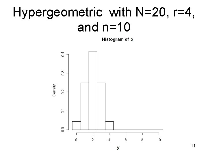
Hypergeometric with N=20, r=4, and n=10 11

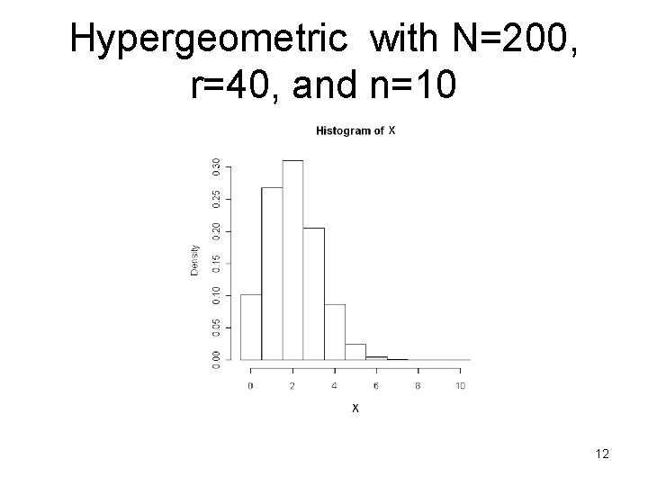
Hypergeometric with N=200, r=40, and n=10 12

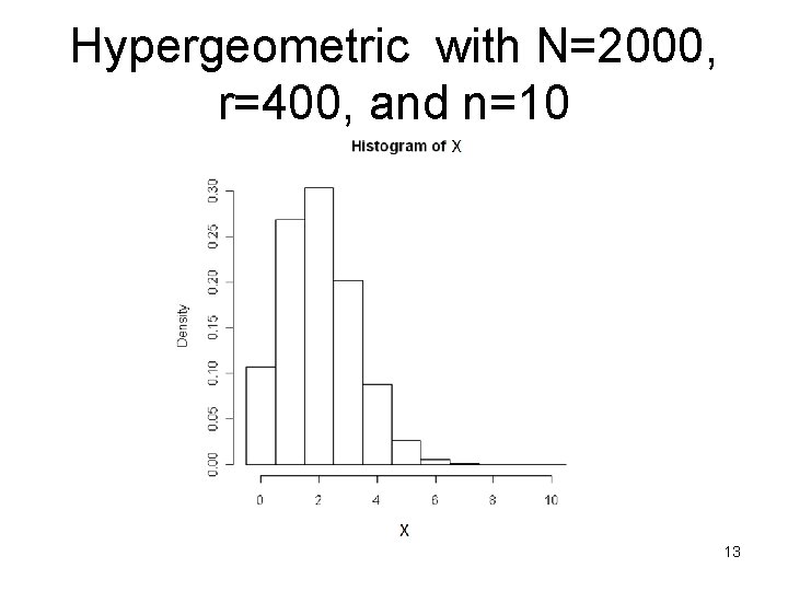
Hypergeometric with N=2000, r=400, and n=10 13

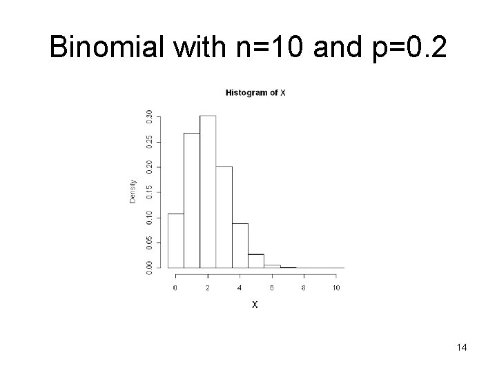
Binomial with n=10 and p=0. 2 14

Epilepsy study http: //www. huffingtonpost. com/hal-herzog/pets-children 15 -epilepsy-sudden-death_b_1791328. html

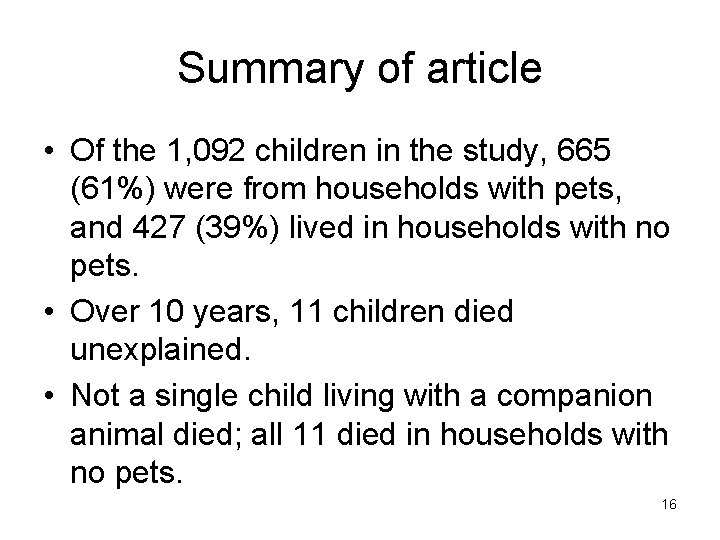
Summary of article • Of the 1, 092 children in the study, 665 (61%) were from households with pets, and 427 (39%) lived in households with no pets. • Over 10 years, 11 children died unexplained. • Not a single child living with a companion animal died; all 11 died in households with no pets. 16

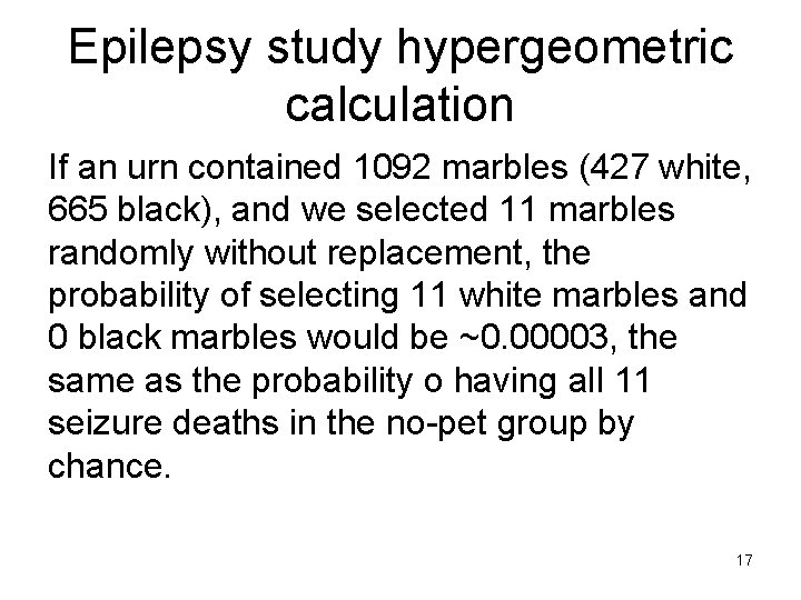
Epilepsy study hypergeometric calculation If an urn contained 1092 marbles (427 white, 665 black), and we selected 11 marbles randomly without replacement, the probability of selecting 11 white marbles and 0 black marbles would be ~0. 00003, the same as the probability o having all 11 seizure deaths in the no-pet group by chance. 17

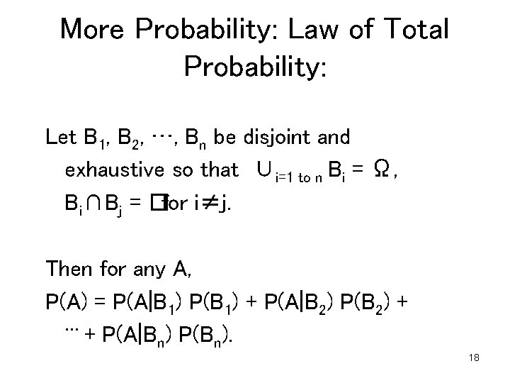
More Probability: Law of Total Probability: Let B 1, B 2, …, Bn be disjoint and exhaustive so that ∪i=1 to n Bi = Ω, Bi∩Bj = �for i≠j. Then for any A, P(A) = P(A|B 1) P(B 1) + P(A|B 2) P(B 2) + … + P(A|B ) P(B ). n n 18

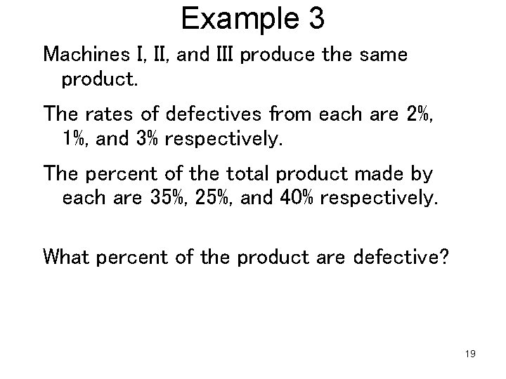
Example 3 Machines I, II, and III produce the same product. The rates of defectives from each are 2%, 1%, and 3% respectively. The percent of the total product made by each are 35%, 25%, and 40% respectively. What percent of the product are defective? 19

Example 3 Workspace 20

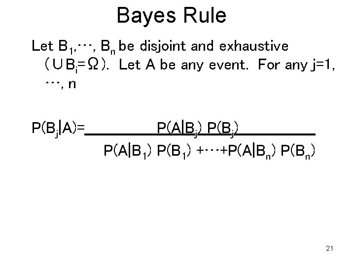
Bayes Rule Let B 1, …, Bn be disjoint and exhaustive (∪Bi=Ω). Let A be any event. For any j=1, …, n P(Bj|A)= P(A|Bj) P(A|B 1) P(B 1) +…+P(A|Bn) P(Bn) 21

Example 3 revisited • What is the probability that a randomly chosen defective was produced by machine 3? 22

Probability Pt. II – Discrete Random Variables A random variable is a function that assigns a numerical value to each sample point. 23

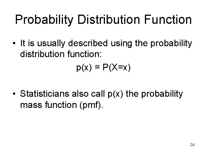
Probability Distribution Function • It is usually described using the probability distribution function: p(x) = P(X=x) • Statisticians also call p(x) the probability mass function (pmf). 24

Cumulative Distribution Function • It is also often described using the cumulative distribution function (c. d. f. ) • F(x) = P(X≤x) 25

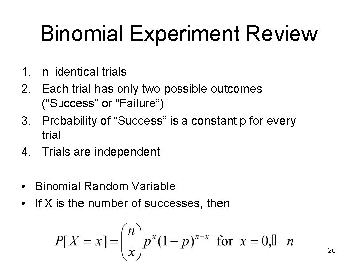
Binomial Experiment Review 1. n identical trials 2. Each trial has only two possible outcomes (“Success” or “Failure”) 3. Probability of “Success” is a constant p for every trial 4. Trials are independent • Binomial Random Variable • If X is the number of successes, then 26

Hypergeometric Experiment Review 1. Population of size N 2. r are “successes” and N-r are “failures” 3. A random sample of size n is taken without replacement Hypergeometric Random Variable • If X is the number of successes, then 27

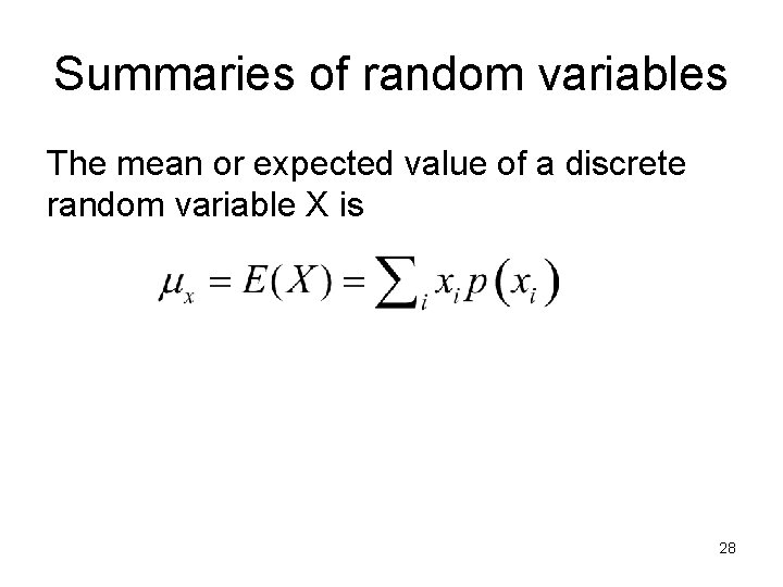
Summaries of random variables The mean or expected value of a discrete random variable X is 28

Expected Value Workspace 29

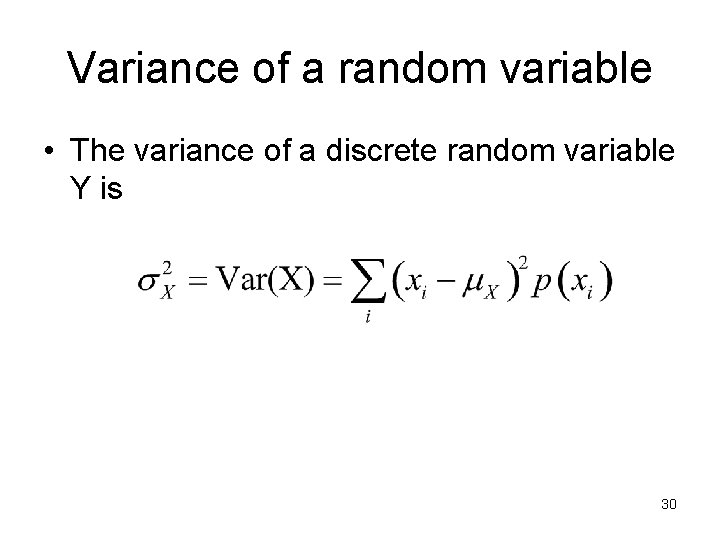
Variance of a random variable • The variance of a discrete random variable Y is 30

Variance Workspace 31

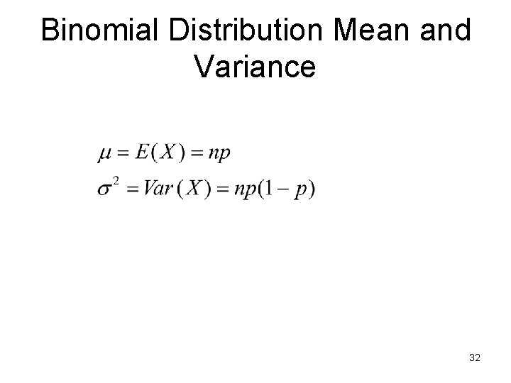
Binomial Distribution Mean and Variance 32

Binomial Distribution Mean and Variance Workspace 33

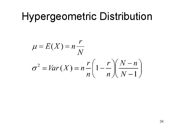
Hypergeometric Distribution 34

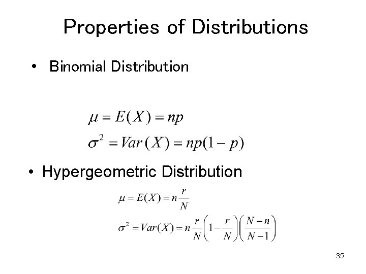
Properties of Distributions • Binomial Distribution • Hypergeometric Distribution 35