Stat 31 Section 1 Last Time Sampling Distributions

Stat 31, Section 1, Last Time Sampling Distributions • Binomial Distribution • Binomial Probs • Normal Approx. to Binomial • Counts Scale vs. Proportion Scale

Important Announcement 2 nd Midterm Date Changed, from: Tuesday, April 5, to Tuesday, April 12.

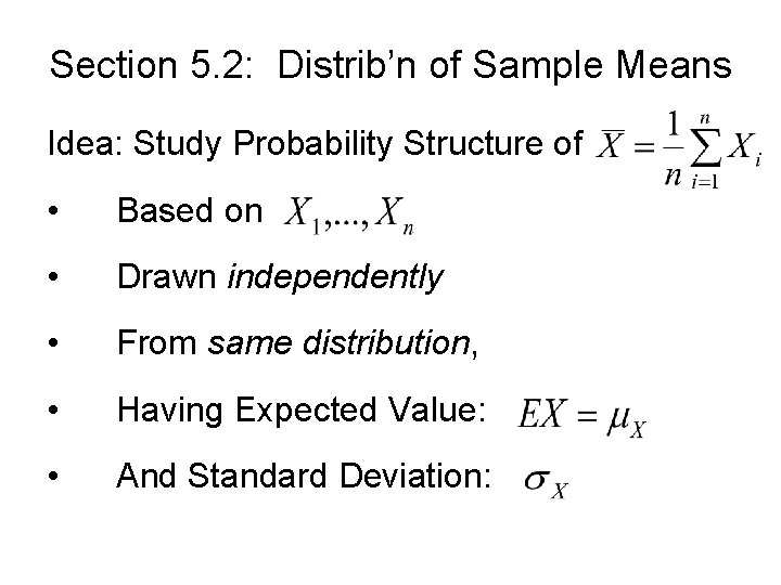
Section 5. 2: Distrib’n of Sample Means Idea: Study Probability Structure of • Based on • Drawn independently • From same distribution, • Having Expected Value: • And Standard Deviation:

Expected Value of Sample Mean How does relate to ? Sample mean “has the same mean” as the original data.

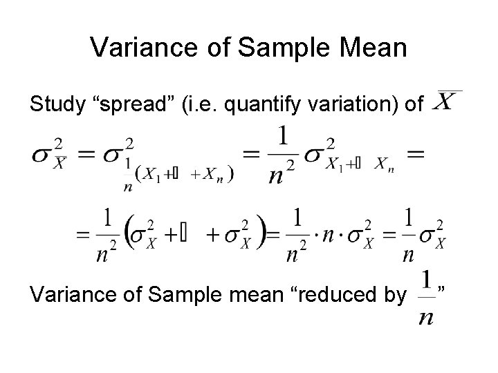
Variance of Sample Mean Study “spread” (i. e. quantify variation) of Variance of Sample mean “reduced by ”

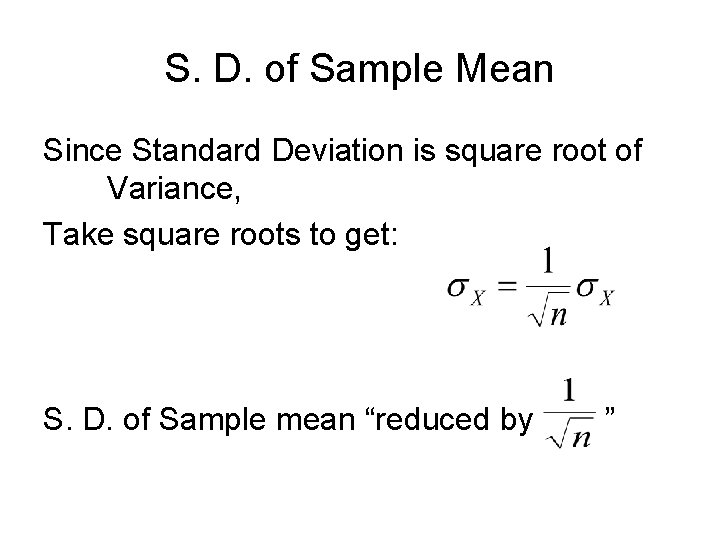
S. D. of Sample Mean Since Standard Deviation is square root of Variance, Take square roots to get: S. D. of Sample mean “reduced by ”

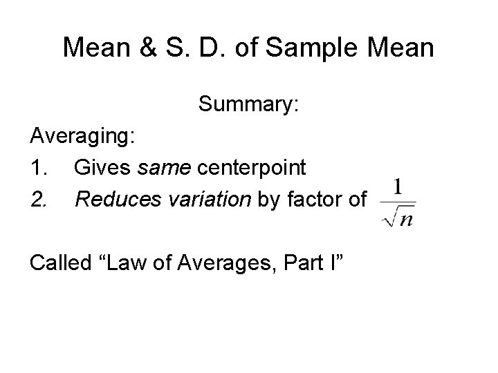
Mean & S. D. of Sample Mean Summary: Averaging: 1. Gives same centerpoint 2. Reduces variation by factor of Called “Law of Averages, Part I”

Law of Averages, Part I Some consequences (worth noting): • To “double accuracy”, need 4 times as much data. • For 10 times accuracy”, need 100 times as much data.

Law of Averages, Part I HW: 5. 28 (5. 77, 4)

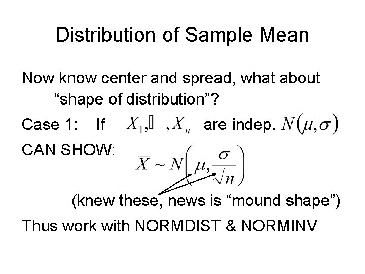
Distribution of Sample Mean Now know center and spread, what about “shape of distribution”? Case 1: If are indep. CAN SHOW: (knew these, news is “mound shape”) Thus work with NORMDIST & NORMINV

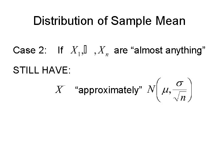
Distribution of Sample Mean Case 2: If are “almost anything” STILL HAVE: “approximately”

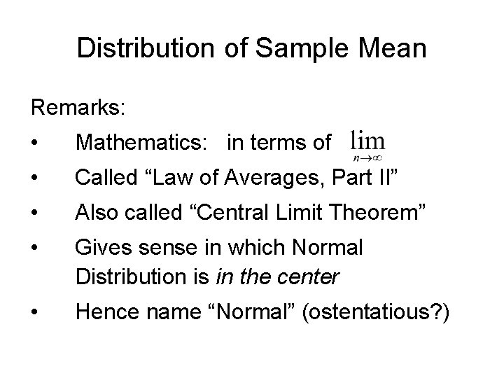
Distribution of Sample Mean Remarks: • Mathematics: in terms of • Called “Law of Averages, Part II” • Also called “Central Limit Theorem” • Gives sense in which Normal Distribution is in the center • Hence name “Normal” (ostentatious? )

Law of Averages, Part II More Remarks: • Thus we will work with NORMDIST & NORMINV a lot, for averages • This is why Normal Dist’n is good model for many different populations (any sum of small indep. Random pieces) • Also explains Normal Approximation to the Binomial

Normal Approx. to Binomial Explained by Law of Averages. II, since: For X ~ Binomial (n. p) Can represent X as: Where: Thus X is an average (rescaled sum), so Law of Averages gives Normal Dist’n

Law of Averages, Part II Nice Java Demo: http: //www. amstat. org/publications/jse/v 6 n 3/applets/CLT. html 1 Dice (think n = 1): 2 Dice (n = 1): Average Dist’n is flat Average Dist’n is triangle … 5 Dice (n = 5): Looks quite “mound shaped”

Law of Averages, Part II Another cool one: http: //www. ruf. rice. edu/~lane/stat_sim/sampling_dist/index. html • Create U shaped distribut’n with mouse • Simul. samples of size 2: non-Normal • Size n = 5: more normal • Size n = 10 or 25: mound shaped

Law of Averages, Part II Class Example: https: //www. unc. edu/~marron/UNCstat 31 -2005/Stat 31 Eg 19. xls Shows: • Even starting from non-normal shape, • Averages become normal • More so for more averaging • SD smaller with more averaging ( )

Law of Averages, Part II HW: 5. 31, 5. 33, 5. 35, 5. 39

And now for something completely different…. A statistics professor was describing sampling theory to his class, explaining how a sample can be studied and used to generalize to a population. ? ? ?

Chapter 6: Statistical Inference Main Idea: Form conclusions by quantifying uncertainty (will study several approaches, first is…)

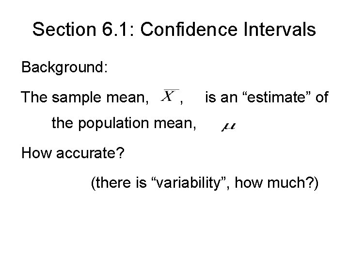
Section 6. 1: Confidence Intervals Background: The sample mean, , is an “estimate” of the population mean, How accurate? (there is “variability”, how much? )

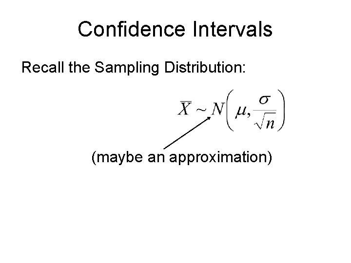
Confidence Intervals Recall the Sampling Distribution: (maybe an approximation)

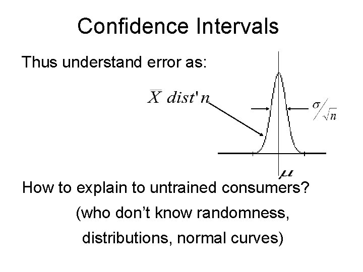
Confidence Intervals Thus understand error as: How to explain to untrained consumers? (who don’t know randomness, distributions, normal curves)

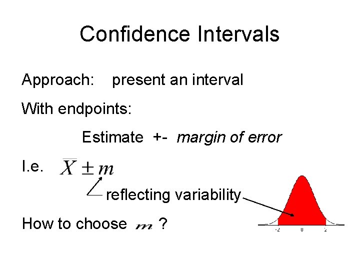
Confidence Intervals Approach: present an interval With endpoints: Estimate +- margin of error I. e. reflecting variability How to choose ?

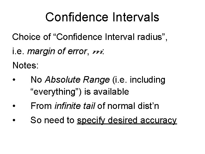
Confidence Intervals Choice of “Confidence Interval radius”, i. e. margin of error, : Notes: • No Absolute Range (i. e. including “everything”) is available • From infinite tail of normal dist’n • So need to specify desired accuracy

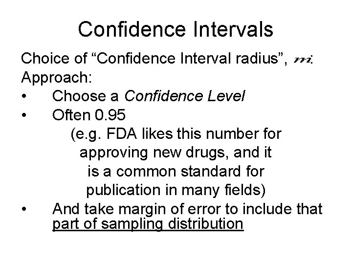
Confidence Intervals Choice of “Confidence Interval radius”, : Approach: • Choose a Confidence Level • Often 0. 95 (e. g. FDA likes this number for approving new drugs, and it is a common standard for publication in many fields) • And take margin of error to include that part of sampling distribution

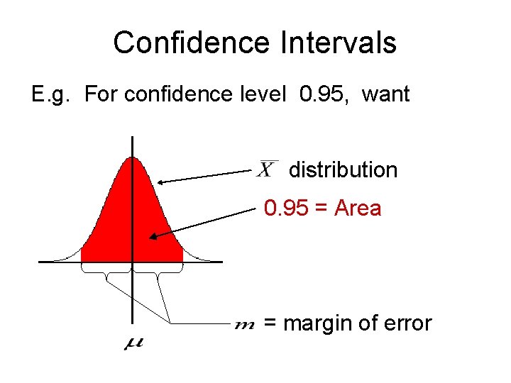
Confidence Intervals E. g. For confidence level 0. 95, want distribution 0. 95 = Area = margin of error

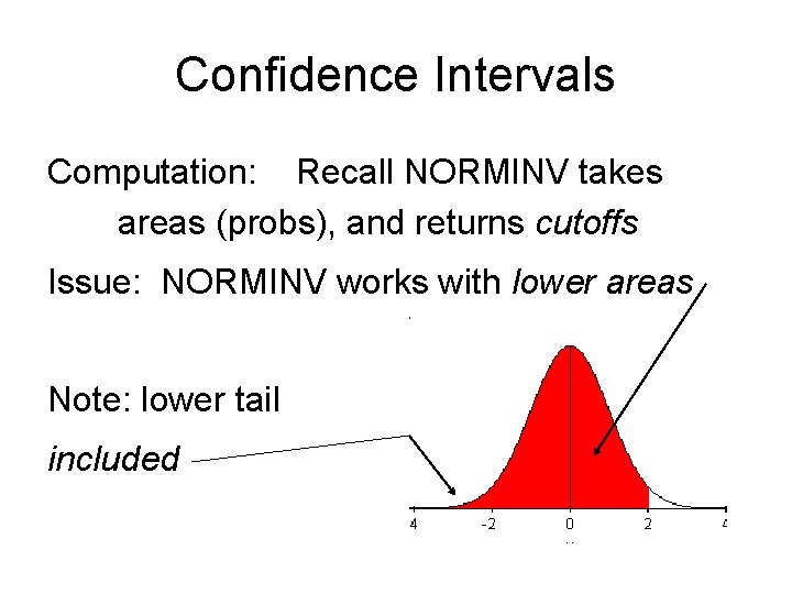
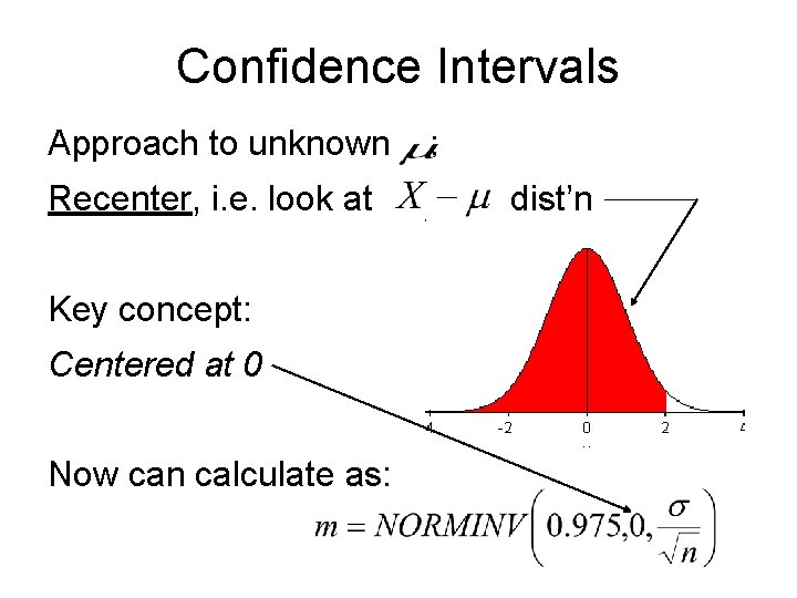
Confidence Intervals Computation: Recall NORMINV takes areas (probs), and returns cutoffs Issue: NORMINV works with lower areas Note: lower tail included

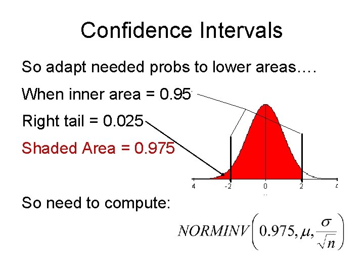
Confidence Intervals So adapt needed probs to lower areas…. When inner area = 0. 95, Right tail = 0. 025 Shaded Area = 0. 975 So need to compute:

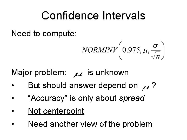
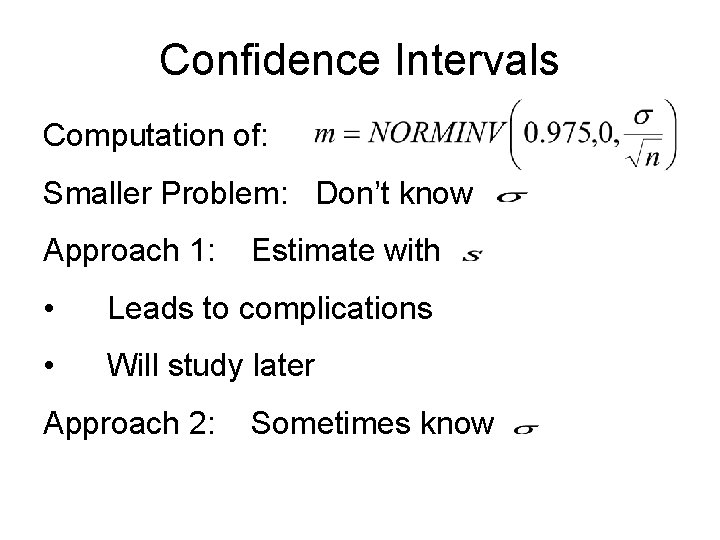
Confidence Intervals Need to compute: Major problem: is unknown • But should answer depend on • “Accuracy” is only about spread • Not centerpoint • Need another view of the problem ?

Confidence Intervals Approach to unknown Recenter, i. e. look at Key concept: Centered at 0 Now can calculate as: : dist’n

Confidence Intervals Computation of: Smaller Problem: Don’t know Approach 1: Estimate with • Leads to complications • Will study later Approach 2: Sometimes know

Confidence Intervals 138 E. g. Crop researchers plant 15 plots 139. 1 113 with a new variety of corn. The 132. 5 yields, in bushels per acre are: 109. 7 140. 7 118. 9 134. 8 109. 6 Assume that = 10 bushels / acre 127. 3 115. 6 130. 4 130. 2 111. 7 105. 5

Confidence Intervals E. g. Find: a) The 90% Confidence Interval for the mean value , for this type of corn. b) The 95% Confidence Interval. c) The 99% Confidence Interval. d) How do the CIs change as the confidence level increases? Solution, part 1 of: https: //www. unc. edu/~marron/UNCstat 31 -2005/Stat 31 Eg 20. xls

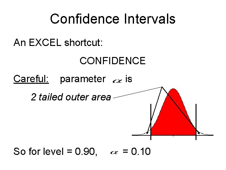
Confidence Intervals An EXCEL shortcut: CONFIDENCE Careful: parameter is: 2 tailed outer area So for level = 0. 90, = 0. 10

Confidence Intervals HW: 6. 1, 6. 3, 6. 5