Stat 31 Section 1 Last Time Random Variables

Stat 31, Section 1, Last Time Random Variables: • Means • Expected Value • Variance • Standard Deviation

Chapter 5 Sampling Distributions Idea: Extend probability tools to distributions we care about: (i) Counts in Political Polls (ii) Measurement Error

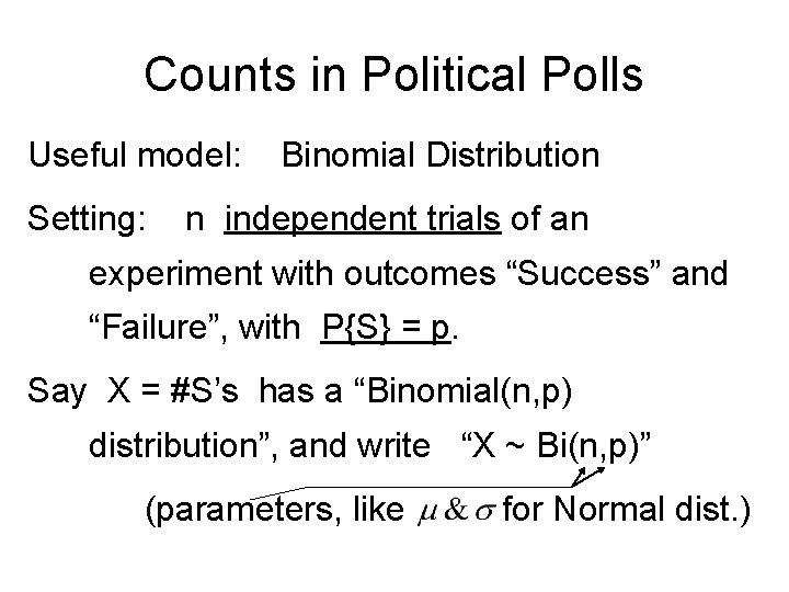
Counts in Political Polls Useful model: Setting: Binomial Distribution n independent trials of an experiment with outcomes “Success” and “Failure”, with P{S} = p. Say X = #S’s has a “Binomial(n, p) distribution”, and write “X ~ Bi(n, p)” (parameters, like for Normal dist. )

Binomial Distributions Models much more than political polls: E. g. Coin tossing (recall saw “independence” was good) E. g. Shooting free throws (in basketball) • Is p always the same? • Really independent? (turns out to be OK)

Binomial Distributions HW on Binomial Assumptions: 5. 1, 5. 3

Binomial Distributions Could work out a formula for Binomial Probs, but results are summarized in Excel function: BINOMDIST Example of Use: https: //www. unc. edu/~marron/UNCstat 31 -2005/Stat 31 Eg 17. xls

Binomial Probs in EXCEL To compute P{X=x}, x n p for X ~ Bi(n, p):

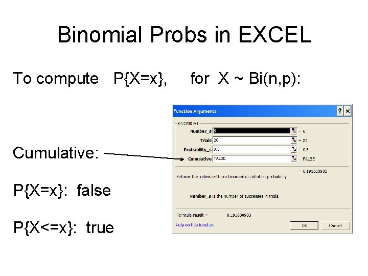
Binomial Probs in EXCEL To compute P{X=x}, Cumulative: P{X=x}: false P{X<=x}: true for X ~ Bi(n, p):

Binomial Probs in EXCEL https: //www. unc. edu/~marron/UNCstat 31 -2005/Stat 31 Eg 17. xls Check this spreadsheet for details of other parts, and some important variations

Binomial Probs in EXCEL HW: 5. 5 5. 6 (. 0074, . 01) Rework using Binomial Distribution: 4. 31

Binomial Distribution “Shape” of Binomial Distribution: Use Probability Histogram Just a bar graph, where heights are probabilities Note: connected to previous histogram by frequentist view (via histogram of repeated samples)

Binomial Distribution Study Distribution Shapes using Excel https: //www. unc. edu/~marron/UNCstat 31 -2005/Stat 31 Eg 18. xls Part I: different p, note several ranges of p are shown Part II: different n, note really “live in different areas”

Binomial Distribution A look under the hood https: //www. unc. edu/~marron/UNCstat 31 -2005/Stat 31 Eg 18. xls Create probability histograms by: – Create Column of xs (e. g. B 9: B 29) – Create Probs (using BINOMDIST, C 9: J 29) – Plot with Chart Wizard Click Chart & Chart Wizard Follow steps, check “series” carefully)

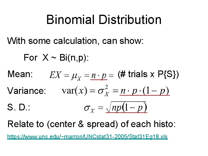
Binomial Distribution With some calculation, can show: For X ~ Bi(n, p): Mean: (# trials x P{S}) Variance: S. D. : Relate to (center & spread) of each histo: https: //www. unc. edu/~marron/UNCstat 31 -2005/Stat 31 Eg 18. xls

Binomial Distribution E. g. : Class HW on %Males at UNC: https: //www. unc. edu/~marron/UNCstat 31 -2005/Stat 31 Eg 16. xls Note Theoretical Means in E 115: H 115, Compare to Sample Means in E 110: H 110: Q 1: Sample Mean smaller – course not representative Q 2: Sample Mean bigger – bias toward males Q 3: Sample Mean bigger – bias toward males Q 4: Sample Mean close Which differences are “significant”?

Binomial Distribution E. g. : Class HW on %Males at UNC: https: //www. unc. edu/~marron/UNCstat 31 -2005/Stat 31 Eg 16. xls Note Theoretical SDs in E 116: H 115, 6 Compare to Sample SDs in E 112: H 112: Q 1: Sample SDs smaller – course population smaller Q 2: Sample SDs bigger – variety of doors (different p) Q 3: Sample SDs bigger – variety of choices (diff. p? ) Q 4: Sample SDs close Which differences are “significant”?

Binomial Distribution E. g. : Class HW on %Males at UNC: https: //www. unc. edu/~marron/UNCstat 31 -2005/Stat 31 Eg 16. xls Probability Histograms (see 3 rd column of plots), Good view of above ideas (for samples): Q 1: mean too small, not enough spread Q 2: mean too big, too spread Q 3: mean too big, too spread Q 4: looks “about right”…

Binomial Distribution HW: 5. 17 5. 19

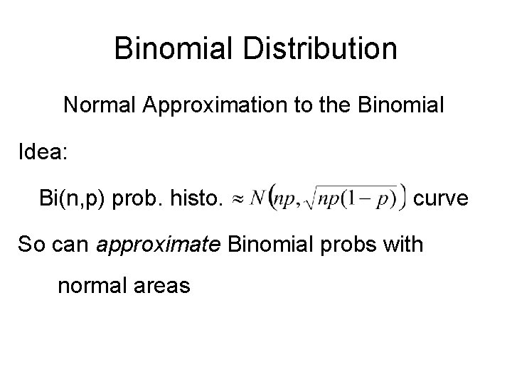
Binomial Distribution Normal Approximation to the Binomial Idea: Bi(n, p) prob. histo. curve So can approximate Binomial probs with normal areas

Normal Approx. to Binomial Before modern software, this was a critical issue, since Binomial Table (C in text) only goes to n = 20. Normal Approx made this possible… Now still useful, since BINONDIST conks out around n = 1000 (but political polls need n ~ 2000 -3000).

Normal Approx. to Binomial Visualization of Normal Approximation: https: //www. unc. edu/~marron/UNCstat 31 -2005/Stat 31 Eg 18. xls Bi(100, 0. 3): Looks really good Bi(20, 0. 5): Chunky, approx. a little weak Bi(20, 0. 05): p too small for good approx. Bi(20, 0. 95): p too big for good approx.

Normal Approx. to Binomial When is Normal Approximation “acceptable”? Textbooks “Rule of Thumb” (there are others): Need: np >= 10 and n(1 -p) >= 10 Relate to above examples: Bi(20, 0. 5): np = n(1 -p) = 10, boundary case Bi(20, 0. 05): np = 4 < 10, poor approx. Bi(20, 0. 95): n(1 -p) = 4 < 10, poor approx.

Normal Approx. to Binomial HW: 5. 23 5. 24 (1050, 17. 7, 0. 997, ~0, 0. 298)

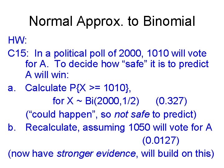
Normal Approx. to Binomial HW: C 15: In a political poll of 2000, 1010 will vote for A. To decide how “safe” it is to predict A will win: a. Calculate P{X >= 1010}, for X ~ Bi(2000, 1/2) (0. 327) (“could happen”, so not safe to predict) b. Recalculate, assuming 1050 will vote for A (0. 0127) (now have stronger evidence, will build on this)

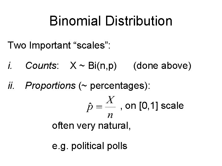
Binomial Distribution Two Important “scales”: i. Counts: ii. Proportions (~ percentages): X ~ Bi(n, p) (done above) , on [0, 1] scale often very natural, e. g. political polls

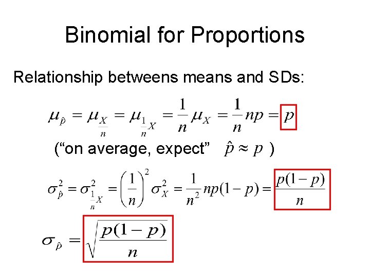
Binomial for Proportions Relationship betweens means and SDs: (“on average, expect” )

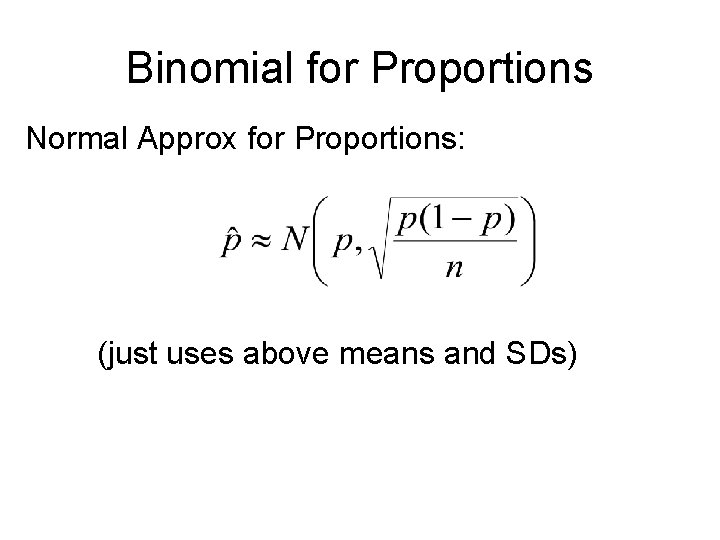
Binomial for Proportions Normal Approx for Proportions: (just uses above means and SDs)

Binomial for Proportions HW: 5. 25 work with both BINOMDIST and Normal Approx.