Stanford Center for Reservoir Forecasting Modeling Geological Scenario

Stanford Center for Reservoir Forecasting Modeling Geological Scenario Uncertainty from Seismic Data using Pattern Similarity Cheolkyun Jeong, Céline Scheidt, Jef Caers, and Tapan Mukerji SCRF 2013

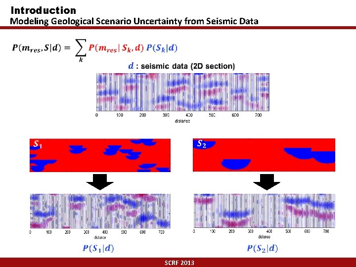
Introduction Modeling Geological Scenario Uncertainty from Seismic Data SCRF 2013

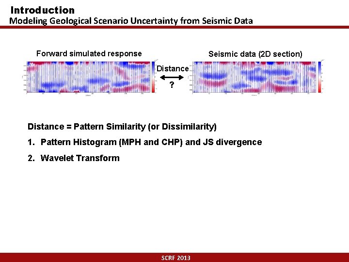
Introduction Modeling Geological Scenario Uncertainty from Seismic Data Forward simulated response Seismic data (2 D section) Distance ? Distance = Pattern Similarity (or Dissimilarity) 1. Pattern Histogram (MPH and CHP) and JS divergence 2. Wavelet Transform SCRF 2013

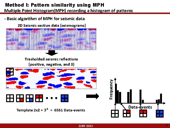
Method I: Pattern similarity using MPH Multiple Point Histogram(MPH) recording a histogram of patterns - Basic algorithm of MPH for seismic data 2 D Seismic section data (seismograms) Frequency Tresholded seismic reflections (positive, negative, and 0) Data-events SCRF 2013 4

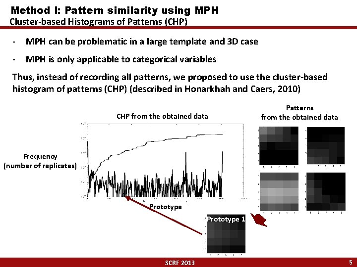
Method I: Pattern similarity using MPH Cluster-based Histograms of Patterns (CHP) - MPH can be problematic in a large template and 3 D case - MPH is only applicable to categorical variables Thus, instead of recording all patterns, we proposed to use the cluster-based histogram of patterns (CHP) (described in Honarkhah and Caers, 2010) CHP from the obtained data Patterns from the obtained data Frequency (number of replicates) Prototype 1 SCRF 2013 5

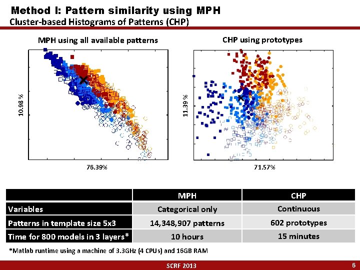
Method I: Pattern similarity using MPH Cluster-based Histograms of Patterns (CHP) CHP using prototypes 11. 39 % 10. 98 % MPH using all available patterns 71. 57% 76. 39% Variables Patterns in template size 5 x 3 Time for 800 models in 3 layers* MPH proportion 30% Categorical only position 20% 14, 348, 907 patterns random 10 hours stacked size CHP # facies red: 20 Continuous light: 2 602 blue: 10 prototypesdark: 3 15 minutes *Matlab runtime using a machine of 3. 3 GHz (4 CPUs) and 16 GB RAM SCRF 2013 6

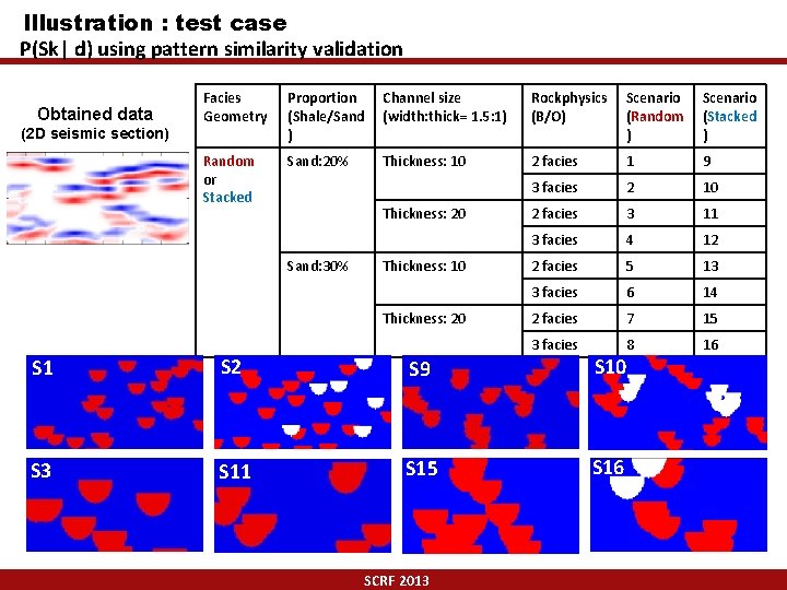
Illustration : test case P(Sk| d) using pattern similarity validation Obtained data (2 D seismic section) Facies Geometry Proportion (Shale/Sand ) Channel size (width: thick= 1. 5: 1) Rockphysics (B/O) Scenario (Random ) Scenario (Stacked ) Random or Stacked Sand: 20% Thickness: 10 2 facies 1 9 3 facies 2 10 2 facies 3 11 3 facies 4 12 2 facies 5 13 3 facies 6 14 2 facies 7 15 3 facies 8 16 Thickness: 20 Sand: 30% Thickness: 10 Thickness: 20 S 1 S 2 S 9 S 10 S 3 S 11 S 15 S 16 SCRF 2013

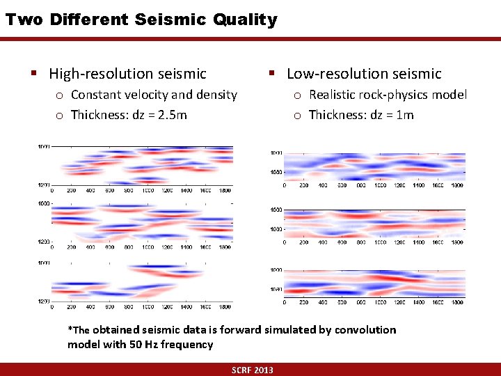
Two Different Seismic Quality § High-resolution seismic § Low-resolution seismic o Constant velocity and density o Thickness: dz = 2. 5 m o Realistic rock-physics model o Thickness: dz = 1 m *The obtained seismic data is forward simulated by convolution model with 50 Hz frequency SCRF 2013

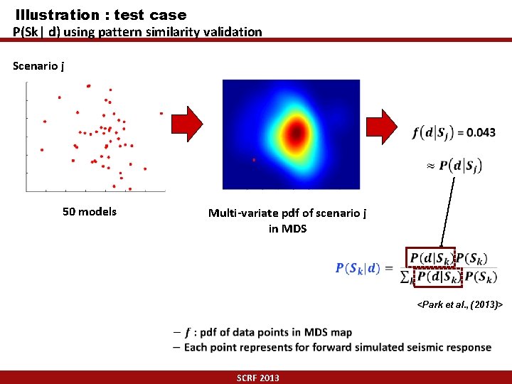
Illustration : test case P(Sk| d) using pattern similarity validation Scenario j 50 models Multi-variate pdf of scenario j in MDS <Park et al. , (2013)> SCRF 2013

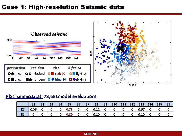
Case 1: High-resolution Seismic data Observed seismic proportion position size # facies 30% stacked red: 20 light: 2 20% random blue: 10 dark: 3 P(Sc|seimicdata): 78, 681 model evaluations KS RS S 1 0. 03 0 S 2 0 0 S 3 0 0 S 4 0 0 S 5 0. 78 0. 80 S 6 0 0 S 7 0 0 S 8 0. 11 0. 10 SCRF 2013 S 9 0 0 S 10 0 0 S 11 0 0 S 12 S 13 S 14 0 0. 07 0 0 0. 10 0 S 15 0 0 S 6 0 0

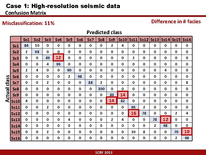
Case 1: High-resolution seismic data Confusion Matrix Difference in # facies Misclassification: 11% Predicted class Actual class Sc 1 Sc 2 Sc 3 Sc 4 Sc 5 Sc 6 Sc 7 Sc 8 Sc 9 Sc 10 Sc 11 Sc 12 Sc 13 Sc 14 Sc 15 Sc 16 Sc 1 84 Sc 2 2 Sc 3 0 Sc 4 0 Sc 5 2 Sc 6 0 Sc 7 0 Sc 8 0 Sc 9 0 Sc 10 4 Sc 11 0 Sc 12 0 Sc 13 0 Sc 14 0 Sc 15 0 Sc 16 0 10 0 0 0 2 4 0 0 0 98 0 0 0 0 86 12 12 0 0 0 4 96 0 0 0 4 0 0 90 0 0 0 0 4 0 0 0 2 98 0 0 0 2 0 0 0 88 2 0 0 0 0 8 0 0 0 100 0 0 0 86 0 0 0 0 14 14 82 0 0 0 0 96 2 0 0 0 0 16 16 78 0 0 2 4 0 0 78 12 12 0 0 0 0 2 98 0 0 0 2 0 0 0 0 10 8 0 0 70 10 10 0 0 0 2 98 SCRF 2013

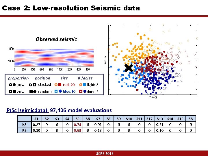
Case 2: Low-resolution Seismic data Observed seismic proportion position size # facies 30% stacked red: 20 light: 2 20% random blue: 10 dark: 3 P(Sc|seimicdata): 97, 406 model evaluations KS RS S 1 0. 27 0. 10 S 2 0 0 S 3 0 0 S 4 0 0 S 5 0. 73 0. 63 S 6 0 0 S 7 0. 01 0. 13 S 8 0 0 SCRF 2013 S 9 0 0 S 10 0 0 S 11 0 0 S 12 S 13 S 14 0 0. 21 0 0 0. 10 0 S 15 0 0 S 6 0 0

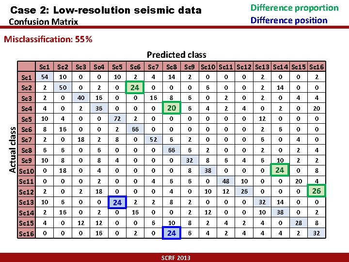
Difference proportion Difference position Case 2: Low-resolution seismic data Confusion Matrix Misclassification: 55% Predicted class Actual class Sc 1 Sc 2 Sc 3 Sc 4 Sc 5 Sc 6 Sc 7 Sc 8 Sc 9 Sc 10 Sc 11 Sc 12 Sc 13 Sc 14 Sc 15 Sc 16 54 10 0 0 10 2 4 14 2 0 0 0 2 2 50 0 24 24 0 0 0 6 0 0 2 14 0 0 2 0 40 16 0 0 16 8 6 0 2 0 4 4 4 0 2 36 0 0 0 20 20 6 4 2 4 0 20 10 4 0 0 72 2 0 0 0 12 0 0 0 8 16 0 0 2 66 0 0 0 2 6 0 0 2 0 18 2 8 0 52 6 2 0 0 0 6 0 4 0 6 6 0 0 0 66 6 2 0 0 2 4 10 8 4 0 0 0 32 8 6 4 6 10 2 2 0 18 0 4 0 0 8 38 0 0 0 24 24 0 8 0 0 0 2 0 0 4 6 6 0 48 10 0 0 20 4 2 0 2 18 0 0 0 4 0 10 12 26 0 0 0 26 26 10 6 0 0 24 24 2 2 8 2 0 0 0 32 14 0 0 2 16 0 2 0 16 0 0 2 12 0 0 10 38 0 2 4 0 12 12 0 0 6 10 8 2 4 0 28 8 0 0 0 16 0 24 24 6 4 2 4 4 4 2 32 SCRF 2013

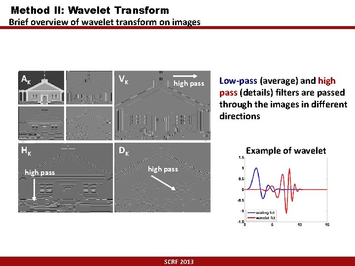
Method II: Wavelet Transform Brief overview of wavelet transform on images AK VK HK DK high pass Low-pass (average) and high pass (details) filters are passed through the images in different directions Example of wavelet high pass SCRF 2013

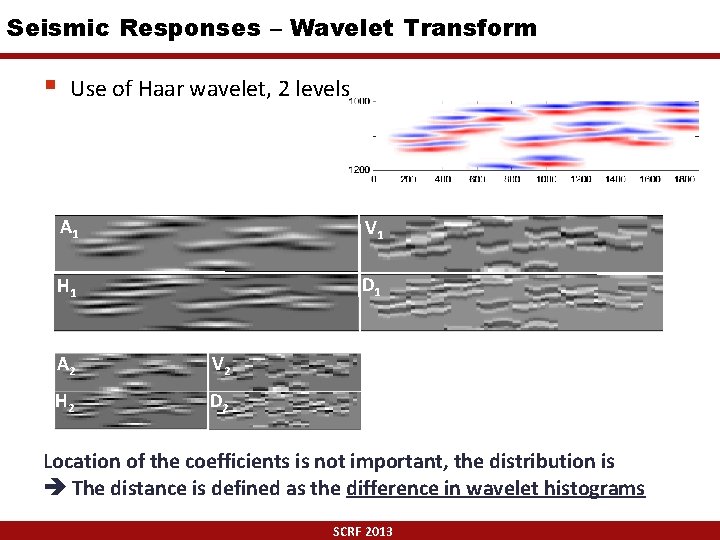
Seismic Responses – Wavelet Transform § Use of Haar wavelet, 2 levels A 1 V 1 H 1 D 1 A 2 V 2 H 2 D 2 Location of the coefficients is not important, the distribution is The distance is defined as the difference in wavelet histograms SCRF 2013

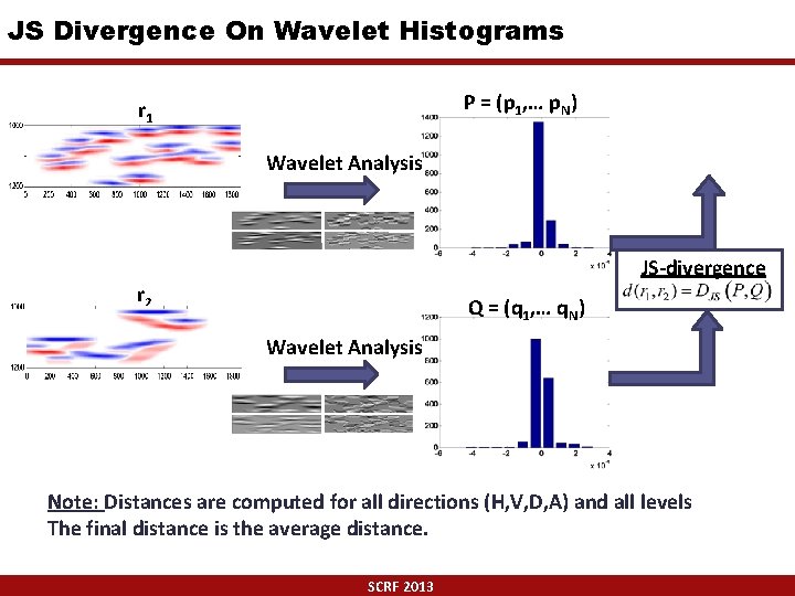
JS Divergence On Wavelet Histograms P = (p 1, … p. N) r 1 Wavelet Analysis JS-divergence r 2 Q = (q 1, … q. N) Wavelet Analysis Note: Distances are computed for all directions (H, V, D, A) and all levels The final distance is the average distance. SCRF 2013

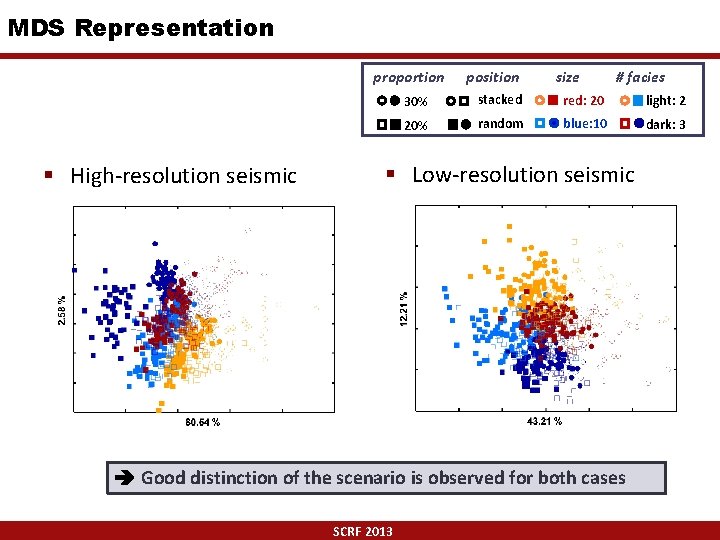
MDS Representation proportion § High-resolution seismic position size # facies 30% stacked red: 20 light: 2 20% random blue: 10 dark: 3 § Low-resolution seismic Good distinction of the scenario is observed for both cases SCRF 2013

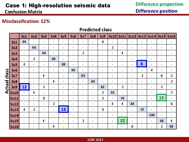
Difference proportion Difference position Case 1: High-resolution seismic data Confusion Matrix Misclassification: 12% Predicted class Actual class Sc 1 Sc 2 Sc 3 Sc 4 Sc 5 Sc 6 Sc 7 Sc 8 Sc 9 Sc 10 Sc 11 Sc 12 Sc 13 Sc 14 Sc 15 Sc 16 Sc 1 94 Sc 2 Sc 3 Sc 4 Sc 5 4 Sc 6 Sc 7 Sc 8 12 Sc 9 12 Sc 10 Sc 11 Sc 12 Sc 13 4 Sc 15 Sc 16 - - - - 98 - - - - 2 - - - - 94 - - - 2 - - - 4 - - - 2 - 98 - - - - 88 - - - - 96 - - - - 4 - - - 86 - - - 2 - 6 2 - - 4 - - - 94 - - - - 2 - - - 82 - - - 2 - 4 - - - 2 92 - - - 8 - - - 2 - 78 - - - 12 12 2 - - - - - 4 4 84 - - - 6 2 - - 16 16 - - - 8 - - - 70 - - - - 100 - - - 4 - - - 22 22 - - - 68 4 - - - - - 6 - - 2 88 SCRF 2013 -

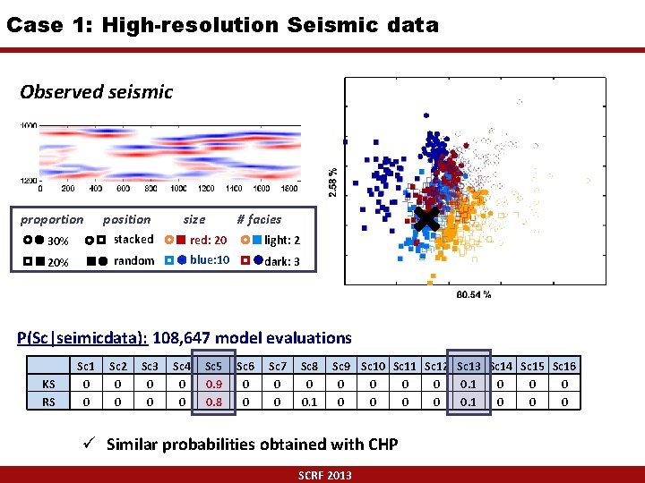
Case 1: High-resolution Seismic data Observed seismic proportion position size # facies 30% stacked red: 20 light: 2 20% random blue: 10 dark: 3 P(Sc|seimicdata): 108, 647 model evaluations KS RS Sc 1 0 0 Sc 2 0 0 Sc 3 0 0 Sc 4 0 0 Sc 5 0. 9 0. 8 Sc 6 0 0 Sc 7 0 0 Sc 8 0 0. 1 Sc 9 Sc 10 Sc 11 Sc 12 Sc 13 Sc 14 Sc 15 Sc 16 0 0 0 0 0. 1 0 0 0 ü Similar probabilities obtained with CHP SCRF 2013

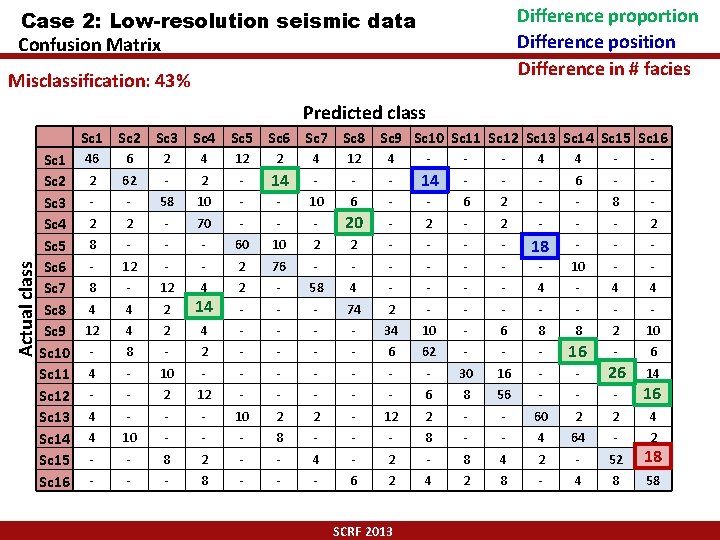
Difference proportion Difference position Difference in # facies Case 2: Low-resolution seismic data Confusion Matrix Misclassification: 43% Predicted class Actual class Sc 1 Sc 2 Sc 3 Sc 4 Sc 5 Sc 6 Sc 7 Sc 8 Sc 9 Sc 10 Sc 11 Sc 12 Sc 13 Sc 14 Sc 15 Sc 16 Sc 1 46 Sc 2 2 Sc 3 Sc 4 2 Sc 5 8 Sc 6 Sc 7 8 Sc 8 4 Sc 9 12 Sc 10 Sc 11 4 Sc 12 Sc 13 4 Sc 14 4 Sc 15 Sc 16 - 6 2 4 12 4 - - - 4 4 - - 62 - 14 14 - - - 6 - - - 58 10 - - 10 6 - - 6 2 - - 8 - 2 - 70 - - - 20 20 - 2 - - - 60 10 2 2 - - 18 18 - - - 12 - - 2 76 - - - - 10 - - - 12 4 - 58 4 - - 4 - 4 4 4 2 14 14 2 - - - 74 2 - - - - 4 2 4 - - 34 10 - 6 8 8 2 10 8 - 2 - - 6 62 - - - 16 16 - 10 - - - - 30 16 - - 26 26 14 - 2 12 - - - 6 8 56 - - - 16 16 - - - 10 2 2 - 12 2 - - 60 2 2 4 10 - - - 8 - - 4 64 - 2 - 8 2 - - 4 - 2 - 8 4 2 - 52 18 18 - - - 6 2 4 2 8 - 4 8 58 SCRF 2013

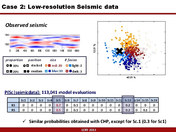
Case 2: Low-resolution Seismic data Observed seismic proportion position size # facies 30% stacked red: 20 light: 2 20% random blue: 10 dark: 3 P(Sc|seimicdata): 113, 041 model evaluations KS RS Sc 1 0 0 Sc 2 0 0 Sc 3 0 0 Sc 4 0 0 Sc 5 0. 7 0. 5 Sc 6 0 0 Sc 7 0. 1 Sc 8 0 0 Sc 9 Sc 10 Sc 11 Sc 12 Sc 13 Sc 14 Sc 15 Sc 16 0 0 0. 2 0 0 0 0. 3 0 0. 1 0 ü Similar probabilities obtained with CHP, except for Sc. 1 (0. 3 for Sc 1) SCRF 2013

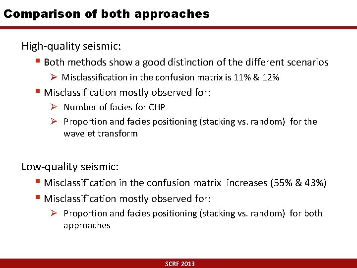
Comparison of both approaches High-quality seismic: § Both methods show a good distinction of the different scenarios Ø Misclassification in the confusion matrix is 11% & 12% § Misclassification mostly observed for: Ø Number of facies for CHP Ø Proportion and facies positioning (stacking vs. random) for the wavelet transform Low-quality seismic: § Misclassification in the confusion matrix § Misclassification mostly observed for: increases (55% & 43%) Ø Proportion and facies positioning (stacking vs. random) for both approaches SCRF 2013

Conclusions & Future work § Successful application of pattern similarity approaches to estimate probabilities of multiple scenarios given observed data • Cluster-based histogram of patterns (CHP) • Wavelet Analysis § Results of distance-based scenario modeling is comparable to rejection sampling for the cases investigated • At only a fraction of the cost § Future work • Application of both pattern similarity approaches to real 3 D case SCRF 2013 23

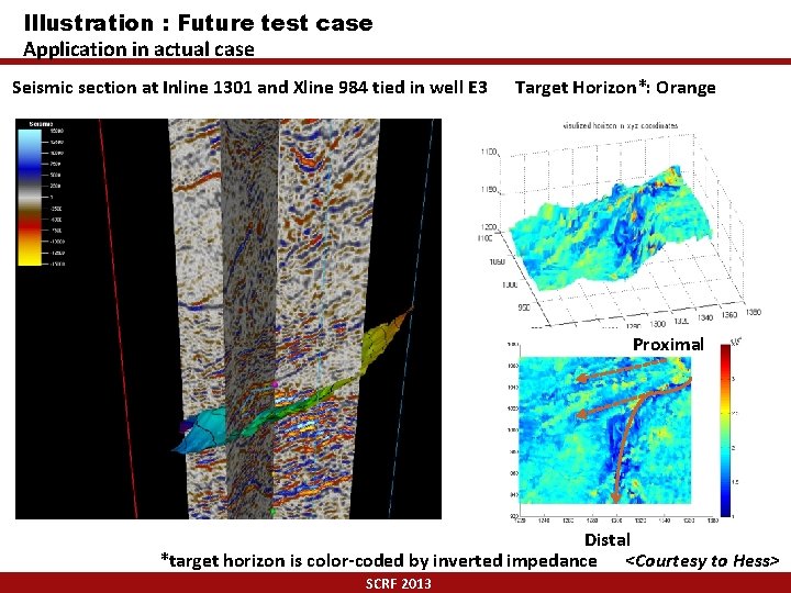
Illustration : Future test case Application in actual case Seismic section at Inline 1301 and Xline 984 tied in well E 3 Target Horizon*: Orange Proximal Distal *target horizon is color-coded by inverted impedance <Courtesy to Hess> SCRF 2013

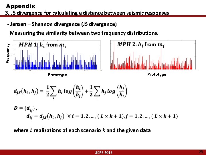
Appendix 3. JS divergence for calculating a distance between seismic responses - Jensen – Shannon divergence (JS divergence) Frequency Measuring the similarity between two frequency distributions. Prototype where L realizations of each scenario k and the given data SCRF 2013 25

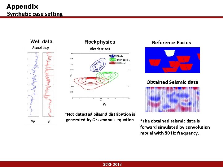
Appendix Synthetic case setting Well data Rockphysics Actual Logs Bivariate pdf Reference Facies Obtained Seismic data Vp Vp *Not detected oilsand distribution is generated by Gassmann’s equation *The obtained seismic data is forward simulated by convolution model with 50 Hz frequency. SCRF 2013