STA 517 Introduction Distribution and Inference 1 4

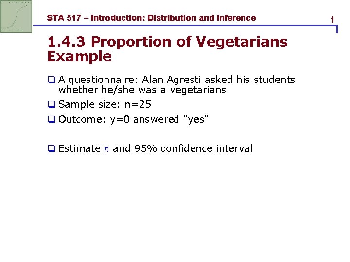
STA 517 – Introduction: Distribution and Inference 1. 4. 3 Proportion of Vegetarians Example q A questionnaire: Alan Agresti asked his students whether he/she was a vegetarians. q Sample size: n=25 q Outcome: y=0 answered “yes” q Estimate and 95% confidence interval 1

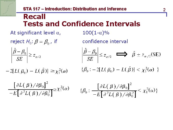
STA 517 – Introduction: Distribution and Inference Recall Tests and Confidence Intervals At significant level , 100(1 - )% reject H 0: confidence interval , if 2

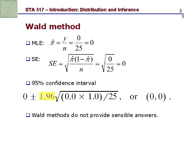
STA 517 – Introduction: Distribution and Inference Wald method q MLE: q SE: q 95% confidence interval q Wald methods do not provide sensible answers. 3

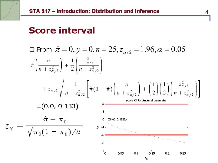
STA 517 – Introduction: Distribution and Inference Score interval q From =(0. 0, 0. 133) 4

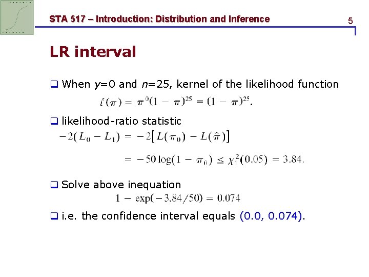
STA 517 – Introduction: Distribution and Inference LR interval q When y=0 and n=25, kernel of the likelihood function q likelihood-ratio statistic q Solve above inequation q i. e. the confidence interval equals (0. 0, 0. 074). 5

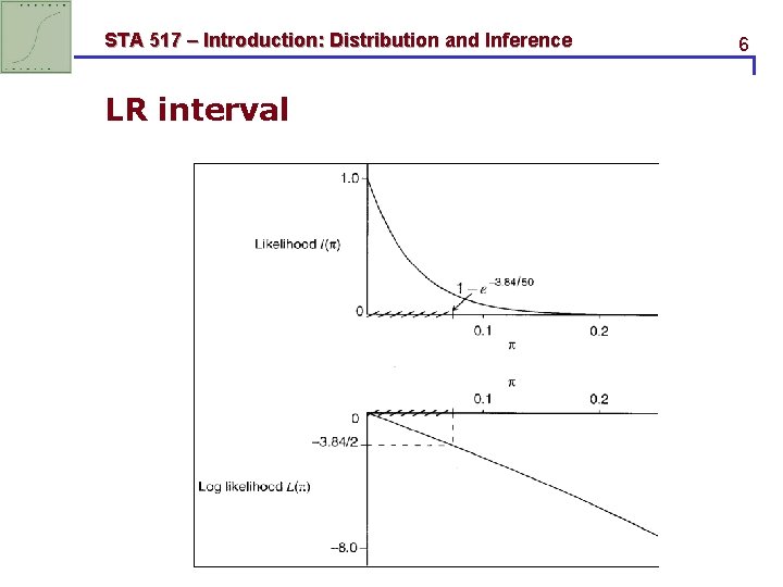
STA 517 – Introduction: Distribution and Inference LR interval 6

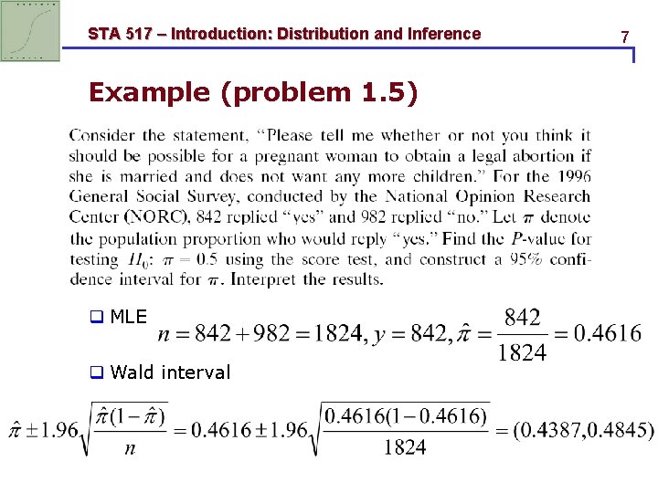
STA 517 – Introduction: Distribution and Inference Example (problem 1. 5) q MLE q Wald interval 7

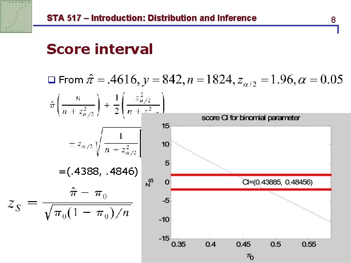
STA 517 – Introduction: Distribution and Inference Score interval q From =(. 4388, . 4846) 8

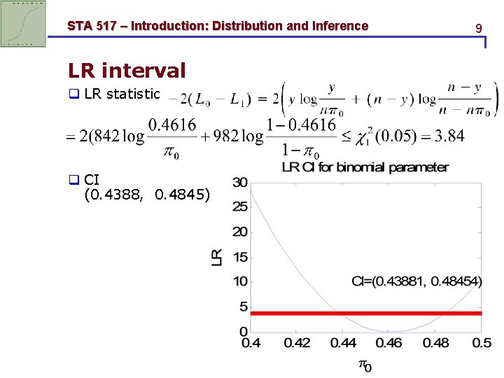
STA 517 – Introduction: Distribution and Inference LR interval q LR statistic q CI (0. 4388, 0. 4845) 9

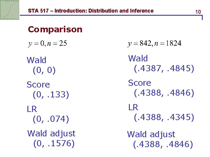
STA 517 – Introduction: Distribution and Inference Comparison Wald (0, 0) Wald (. 4387, . 4845) Score (0, . 133) Score (. 4388, . 4846) LR (0, . 074) LR (. 4388, . 4345) Wald adjust (0, . 1576) Wald adjust (. 4388, . 4846) 10

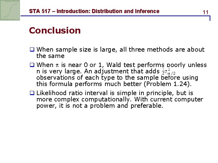
STA 517 – Introduction: Distribution and Inference 11 Conclusion q When sample size is large, all three methods are about the same q When is near 0 or 1, Wald test performs poorly unless n is very large. An adjustment that adds observations of each type to the sample before using this formula performs much better (Problem 1. 24). q Likelihood ratio interval is simple in principle, but is more complex computationally. With current computer power, it is not a problem and preferable.

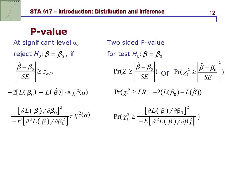
STA 517 – Introduction: Distribution and Inference P-value At significant level , Two sided P-value reject H 0: for test H 0: , if or 12

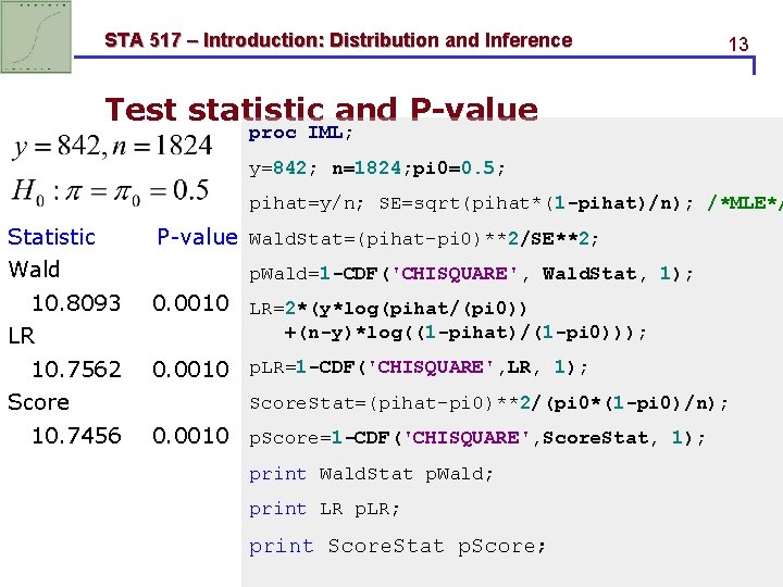
STA 517 – Introduction: Distribution and Inference 13 Test statistic and P-value proc IML; y=842; n=1824; pi 0=0. 5; pihat=y/n; SE=sqrt(pihat*(1 -pihat)/n); /*MLE*/ Statistic Wald 10. 8093 LR 10. 7562 Score 10. 7456 P-value Wald. Stat=(pihat-pi 0)**2/SE**2; p. Wald=1 -CDF('CHISQUARE', Wald. Stat, 1); 0. 0010 LR=2*(y*log(pihat/(pi 0)) +(n-y)*log((1 -pihat)/(1 -pi 0))); 0. 0010 p. LR=1 -CDF('CHISQUARE', LR, 1); Score. Stat=(pihat-pi 0)**2/(pi 0*(1 -pi 0)/n); 0. 0010 p. Score=1 -CDF('CHISQUARE', Score. Stat, 1); print Wald. Stat p. Wald; print LR p. LR; print Score. Stat p. Score;

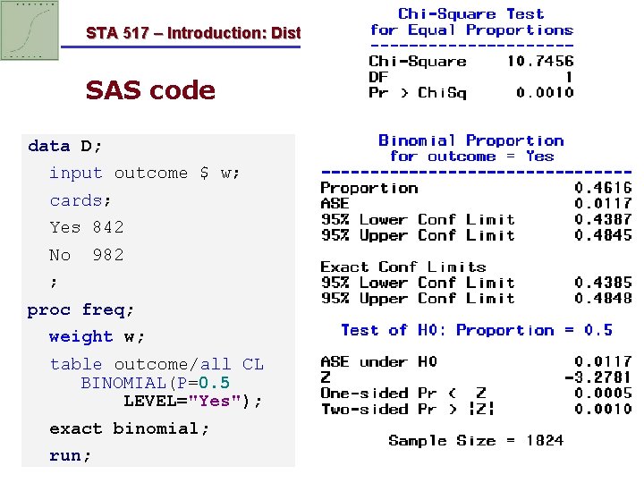
STA 517 – Introduction: Distribution and Inference SAS code data D; input outcome $ w; cards; Yes 842 No 982 ; proc freq; weight w; table outcome/all CL BINOMIAL(P=0. 5 LEVEL="Yes"); exact binomial; run; 14

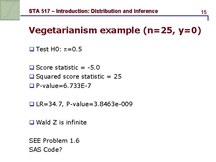
STA 517 – Introduction: Distribution and Inference 15 Vegetarianism example (n=25, y=0) q Test H 0: =0. 5 q Score statistic = -5. 0 q Squared score statistic = 25 q P-value=6. 733 E-7 q LR=34. 7, P-value=3. 8463 e-009 q Wald Z is infinite SEE Problem 1. 6 SAS Code?

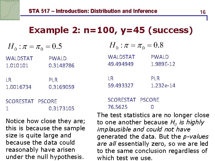
STA 517 – Introduction: Distribution and Inference 16 Example 2: n=100, y=45 (success) WALDSTAT 1. 010101 PWALD 0. 3148786 WALDSTAT 49. 494949 PWALD 1. 989 E-12 LR 1. 0016734 PLR 0. 3169059 LR 59. 493327 PLR 1. 232 e-14 SCORESTAT PSCORE 1 0. 3173105 Notice how close they are; this is because the sample size is quite large and because the data could reasonably have arisen under the null hypothesis. SCORESTAT PSCORE 76. 5625 0 The test statistics are no longer close to one another because H 0 is highly implausible and could not have generated the data. But the p-values are all essentially zero, so we are led to the same conclusion regardless of which test we use.

STA 517 – Introduction: Distribution and Inference 1. 4. 4 Exact Small-Sample Inference q With modern computational power, it is not necessary to rely on large-sample approximations for the distribution of statistics such as ˆ. q Tests and confidence intervals can use the binomial distribution directly rather than its normal approximation. q Such inferences occur naturally for small samples, but apply for any n. 17

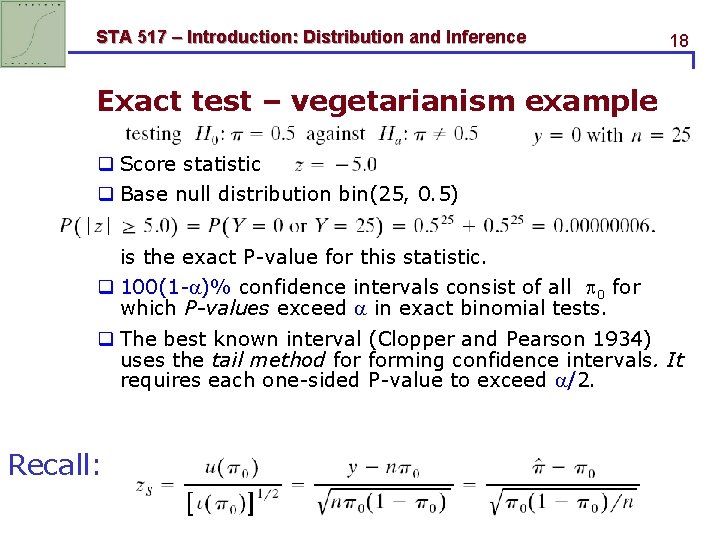
STA 517 – Introduction: Distribution and Inference 18 Exact test – vegetarianism example q Score statistic q Base null distribution bin(25, 0. 5) is the exact P-value for this statistic. q 100(1 - )% confidence intervals consist of all 0 for which P-values exceed in exact binomial tests. q The best known interval (Clopper and Pearson 1934) uses the tail method forming confidence intervals. It requires each one-sided P-value to exceed /2. Recall:

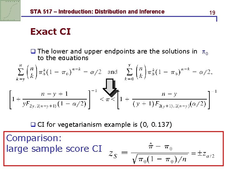
STA 517 – Introduction: Distribution and Inference Exact CI q The lower and upper endpoints are the solutions in 0 to the equations q CI for vegetarianism example is (0, 0. 137) Comparison: large sample score CI 19

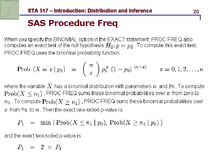
STA 517 – Introduction: Distribution and Inference SAS Procedure Freq 20

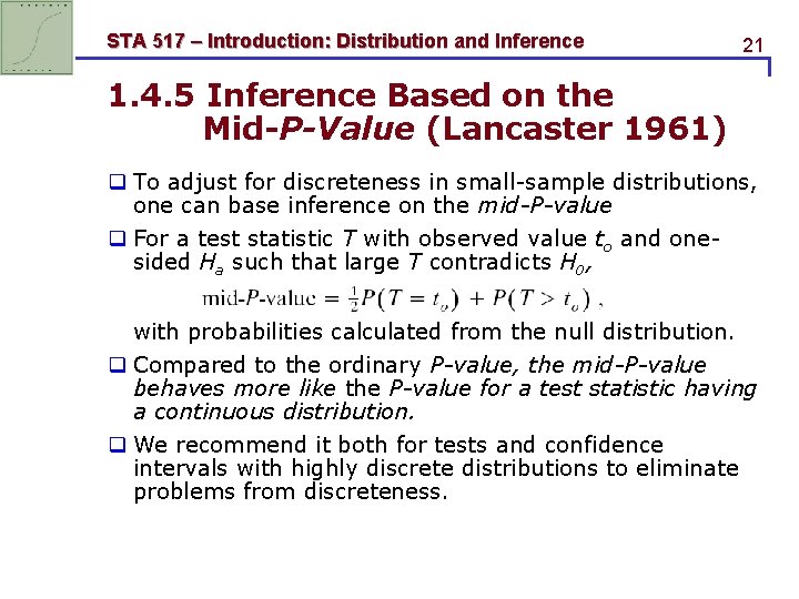
STA 517 – Introduction: Distribution and Inference 21 1. 4. 5 Inference Based on the Mid-P-Value (Lancaster 1961) q To adjust for discreteness in small-sample distributions, one can base inference on the mid-P-value q For a test statistic T with observed value to and onesided Ha such that large T contradicts H 0, with probabilities calculated from the null distribution. q Compared to the ordinary P-value, the mid-P-value behaves more like the P-value for a test statistic having a continuous distribution. q We recommend it both for tests and confidence intervals with highly discrete distributions to eliminate problems from discreteness.

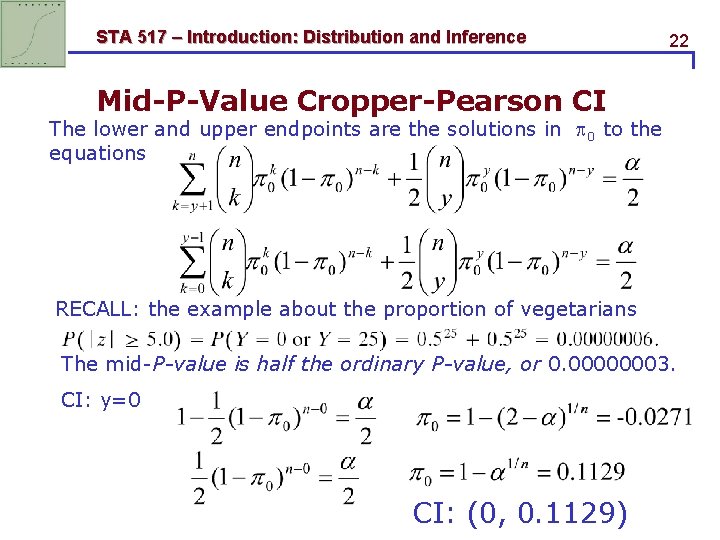
STA 517 – Introduction: Distribution and Inference 22 Mid-P-Value Cropper-Pearson CI The lower and upper endpoints are the solutions in 0 to the equations RECALL: the example about the proportion of vegetarians The mid-P-value is half the ordinary P-value, or 0. 00000003. CI: y=0 CI: (0, 0. 1129)