Spring 2018 Program Analysis and Verification Lecture 5
![Strongest postcondition calculus By Vadim Plessky (http: //svgicons. sourceforge. net/) [see page for license], Strongest postcondition calculus By Vadim Plessky (http: //svgicons. sourceforge. net/) [see page for license],](https://slidetodoc.com/presentation_image_h2/857375281c873d7f27968f9d1e595abc/image-22.jpg)
![Floyd’s strongest postcondition rule v. x=a[v/x] �P[v/x] } [ass. Floyd] { P } x Floyd’s strongest postcondition rule v. x=a[v/x] �P[v/x] } [ass. Floyd] { P } x](https://slidetodoc.com/presentation_image_h2/857375281c873d7f27968f9d1e595abc/image-24.jpg)
![Floyd’s strongest postcondition rule v. x=a[v/x] �P[v/x] } [ass. Floyd] { P } x Floyd’s strongest postcondition rule v. x=a[v/x] �P[v/x] } [ass. Floyd] { P } x](https://slidetodoc.com/presentation_image_h2/857375281c873d7f27968f9d1e595abc/image-25.jpg)
![Conjunction rule {P}S{Q} { P’ } S { Q’ } [conjp] { P �P’ Conjunction rule {P}S{Q} { P’ } S { Q’ } [conjp] { P �P’](https://slidetodoc.com/presentation_image_h2/857375281c873d7f27968f9d1e595abc/image-34.jpg)
![More useful rules {P}C{Q} { P’ } C { Q’ } [disjp] { P More useful rules {P}C{Q} { P’ } C { Q’ } [disjp] { P](https://slidetodoc.com/presentation_image_h2/857375281c873d7f27968f9d1e595abc/image-35.jpg)
![Invariance + Conjunction = Constancy {P}C{Q} [constancyp] { F �P } C { F Invariance + Conjunction = Constancy {P}C{Q} [constancyp] { F �P } C { F](https://slidetodoc.com/presentation_image_h2/857375281c873d7f27968f9d1e595abc/image-36.jpg)
![“Small” assignment axiom [assfloyd] { x=v } x: =a { x=a[v/x] } where v� “Small” assignment axiom [assfloyd] { x=v } x: =a { x=a[v/x] } where v�](https://slidetodoc.com/presentation_image_h2/857375281c873d7f27968f9d1e595abc/image-39.jpg)
![“Small” assignment axiom [assfloyd] { x=v } x: =a { x=a[v/x] } where v� “Small” assignment axiom [assfloyd] { x=v } x: =a { x=a[v/x] } where v�](https://slidetodoc.com/presentation_image_h2/857375281c873d7f27968f9d1e595abc/image-40.jpg)
![“Small” assignment axiom [assfloyd] { x=v } x: =a { x=a[v/x] } where v� “Small” assignment axiom [assfloyd] { x=v } x: =a { x=a[v/x] } where v�](https://slidetodoc.com/presentation_image_h2/857375281c873d7f27968f9d1e595abc/image-41.jpg)
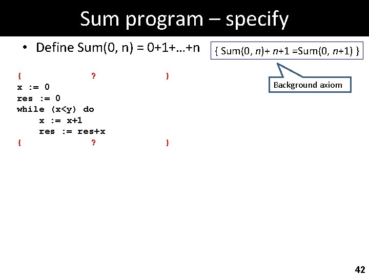

- Slides: 55

Spring 2018 Program Analysis and Verification Lecture 5: Axiomatic Semantics III Predicate Transformer Calculi Roman Manevich Ben-Gurion University

Tentative syllabus Program Verification Program Analysis Basics Abstract Interpretation fundamentals Analysis Techniques Operational semantics Control Flow Graphs Lattices Numerical Domains Hoare Logic Equation Systems Fixed-Points Alias analysis Predicate Calculus Collecting Semantics Chaotic Iteration Interprocedural Analysis Proving Termination Using Soot Galois Connections Shape Analysis Domain constructors CEGAR Data structures Widening/ Narrowing 2

Previously • Hoare logic – Inference system – Annotated programs – Soundness and completeness 3

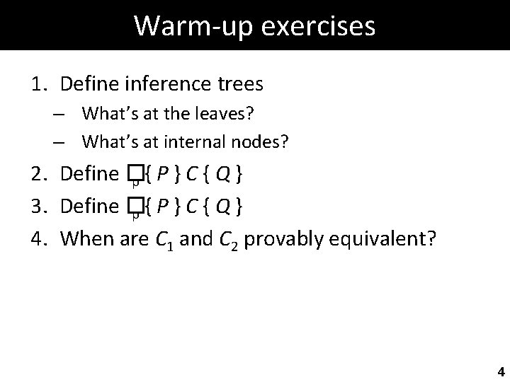
Warm-up exercises 1. Define inference trees – What’s at the leaves? – What’s at internal nodes? 2. Define � p{P}C{Q} 3. Define � p{P}C{Q} 4. When are C 1 and C 2 provably equivalent? 4

Agenda • Weakest precondition • Strongest postcondition • Some useful rules 5

Predicate transformer calculi 6

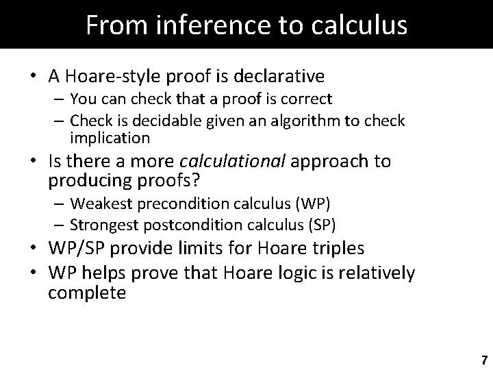
From inference to calculus • A Hoare-style proof is declarative – You can check that a proof is correct – Check is decidable given an algorithm to check implication • Is there a more calculational approach to producing proofs? – Weakest precondition calculus (WP) – Strongest postcondition calculus (SP) • WP/SP provide limits for Hoare triples • WP helps prove that Hoare logic is relatively complete 7

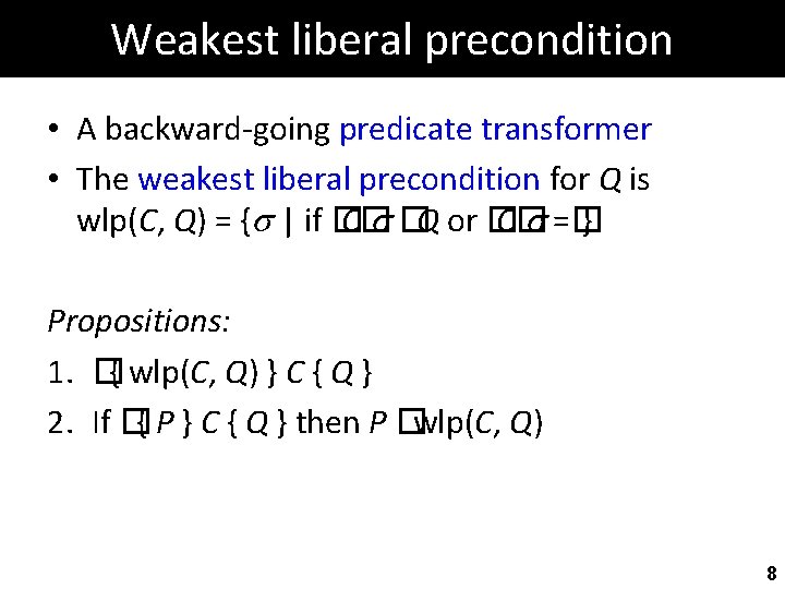
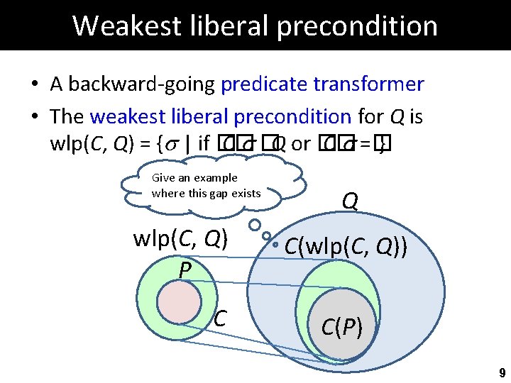
Weakest liberal precondition • A backward-going predicate transformer • The weakest liberal precondition for Q is wlp(C, Q) = { | if � C� �Q or � C� =� } Propositions: 1. �{ wlp(C, Q) } C { Q } 2. If �{ P } C { Q } then P �wlp(C, Q) 8

Weakest liberal precondition • A backward-going predicate transformer • The weakest liberal precondition for Q is wlp(C, Q) = { | if � C� �Q or � C� =� } Give an example where this gap exists wlp(C, Q) P C Q C(wlp(C, Q)) C(P) 9

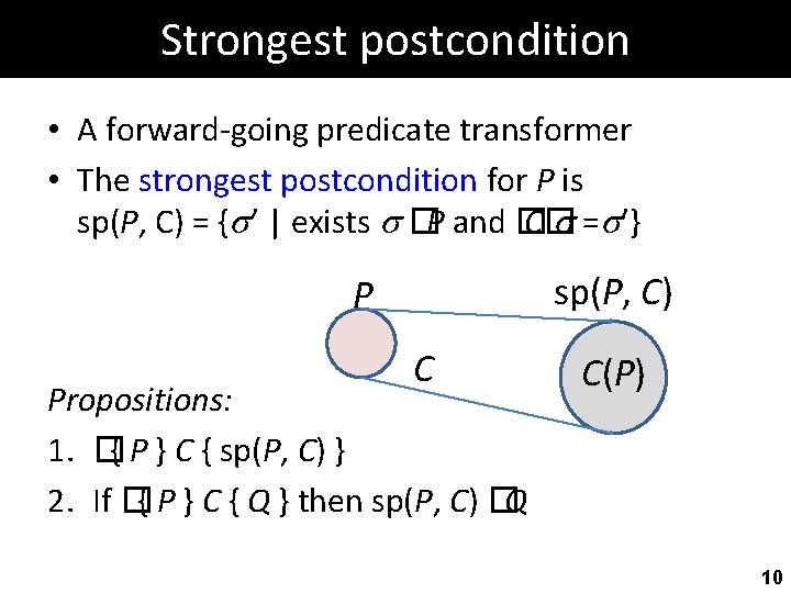
Strongest postcondition • A forward-going predicate transformer • The strongest postcondition for P is sp(P, C) = { ’ | exists �P and � C� = ’} sp(P, C) P C Propositions: 1. �{ P } C { sp(P, C) } 2. If �{ P } C { Q } then sp(P, C) �Q C(P) 10

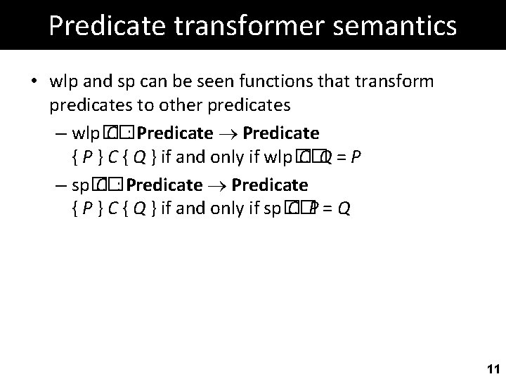
Predicate transformer semantics • wlp and sp can be seen functions that transform predicates to other predicates – wlp� C�: Predicate { P } C { Q } if and only if wlp� C�Q = P – sp� C�: Predicate { P } C { Q } if and only if sp� C�P = Q 11

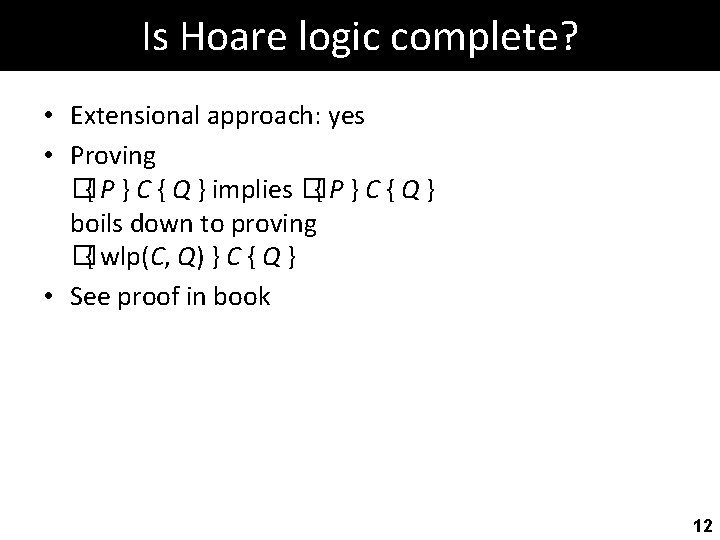
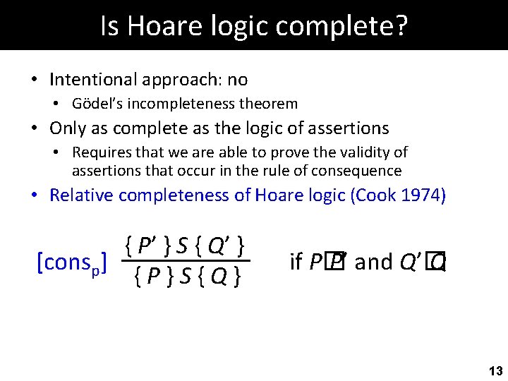
Is Hoare logic complete? • Extensional approach: yes • Proving �{ P } C { Q } implies �{ P } C { Q } boils down to proving �{ wlp(C, Q) } C { Q } • See proof in book 12

Is Hoare logic complete? • Intentional approach: no • Gödel’s incompleteness theorem • Only as complete as the logic of assertions • Requires that we are able to prove the validity of assertions that occur in the rule of consequence • Relative completeness of Hoare logic (Cook 1974) { P’ } S { Q’ } [consp] {P}S{Q} if P� P’ and Q’� Q 13

Weakest (liberal) precondition calculus By Vadim Plessky (http: //svgicons. sourceforge. net/) [see page for license], via Wikimedia Commons 14

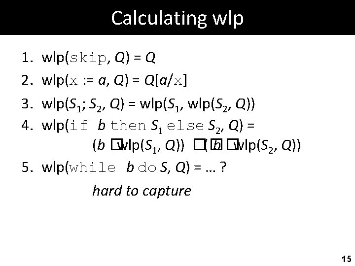
Calculating wlp 1. 2. 3. 4. wlp(skip, Q) = Q wlp(x : = a, Q) = Q[a/x] wlp(S 1; S 2, Q) = wlp(S 1, wlp(S 2, Q)) wlp(if b then S 1 else S 2, Q) = (b �wlp(S 1, Q)) �(� b �wlp(S 2, Q)) 5. wlp(while b do S, Q) = … ? hard to capture 15

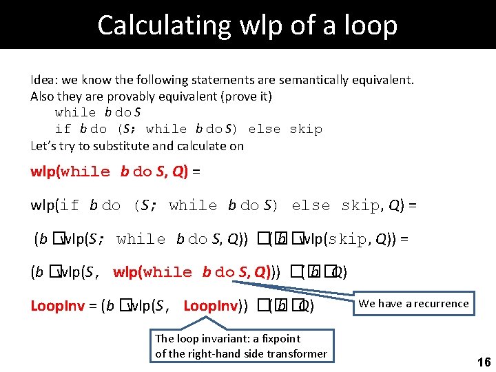
Calculating wlp of a loop Idea: we know the following statements are semantically equivalent. Also they are provably equivalent (prove it) while b do S if b do (S; while b do S) else skip Let’s try to substitute and calculate on wlp(while b do S, Q) = wlp(if b do (S; while b do S) else skip, Q) = (b �wlp(S; while b do S, Q)) �(� b �wlp(skip, Q)) = (b �wlp(S, wlp(while b do S, Q))) �(� b �Q) Loop. Inv = (b �wlp(S, Loop. Inv)) �(� b �Q) The loop invariant: a fixpoint of the right-hand side transformer We have a recurrence 16

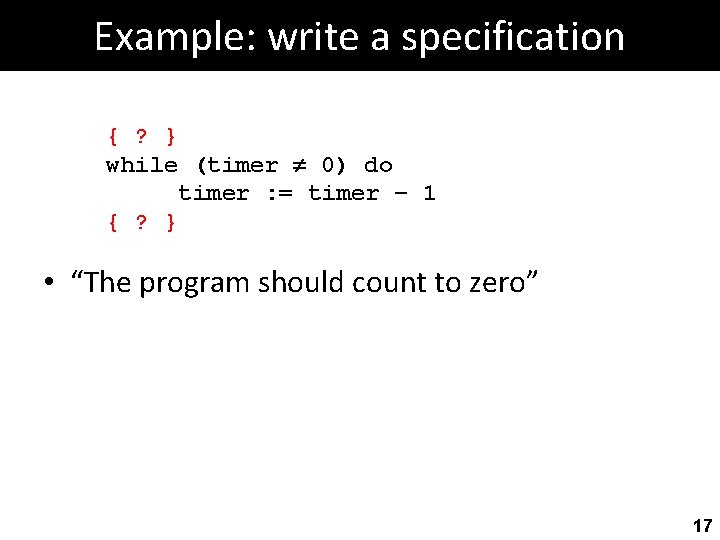
Example: write a specification { ? } while (timer 0) do timer : = timer – 1 { ? } • “The program should count to zero” 17

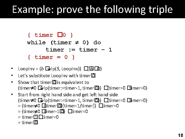
Example: prove the following triple { timer � 0 } while (timer 0) do timer : = timer – 1 { timer = 0 } • Loop. Inv = (b �wlp(S, Loop. Inv)) �(� b �Q) • Let’s substitute Loop. Inv with timer� 0 • Show that timer� 0 is equivalent to (timer 0 �wlp(timer: =timer-1, timer� 0)) �(timer=0 �timer=0) • Start from right hand side and get left hand side (timer 0 �wlp(timer: =timer-1, timer� 0)) �(timer=0 �timer=0) = (timer 0 �(timer� 0)[timer-1/timer]) �timer=0 = (timer 0 �timer-1� 0) �timer=0 = timer� 1 �timer=0 = timer� 0 18

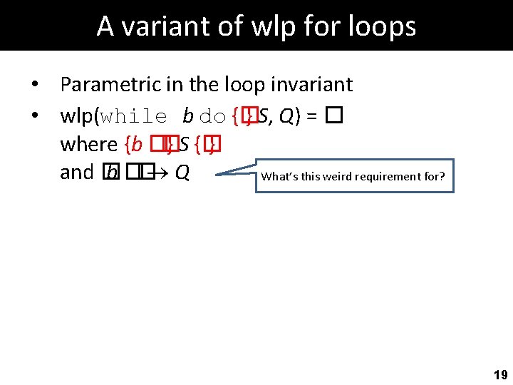
A variant of wlp for loops • Parametric in the loop invariant • wlp(while b do {� } S, Q) = � where {b �� } S {� } and � b �� Q What’s this weird requirement for? 19

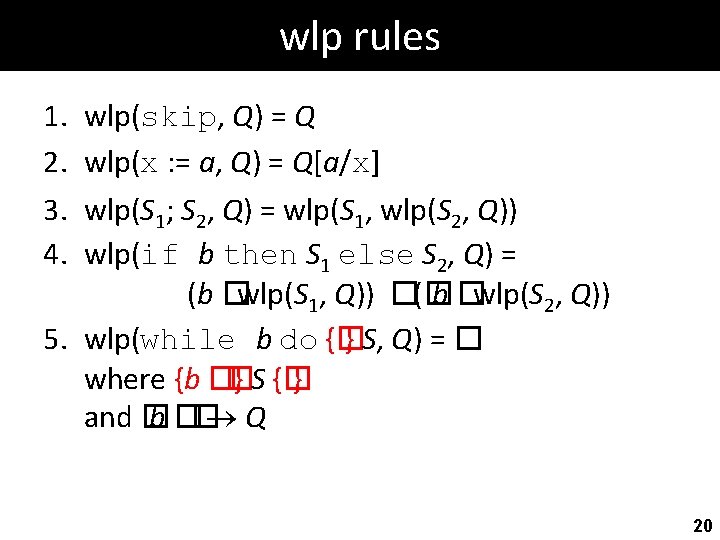
wlp rules 1. 2. 3. 4. wlp(skip, Q) = Q wlp(x : = a, Q) = Q[a/x] wlp(S 1; S 2, Q) = wlp(S 1, wlp(S 2, Q)) wlp(if b then S 1 else S 2, Q) = (b �wlp(S 1, Q)) �(� b �wlp(S 2, Q)) 5. wlp(while b do {� } S, Q) = � where {b �� } S {� } and � b �� Q 20

Issues with wlp-based proofs • Requires backwards reasoning – unintuitive • Backward reasoning is non-deterministic – causes problems when While is extended with dynamically allocated heaps (aliasing) 21
![Strongest postcondition calculus By Vadim Plessky http svgicons sourceforge net see page for license Strongest postcondition calculus By Vadim Plessky (http: //svgicons. sourceforge. net/) [see page for license],](https://slidetodoc.com/presentation_image_h2/857375281c873d7f27968f9d1e595abc/image-22.jpg)
Strongest postcondition calculus By Vadim Plessky (http: //svgicons. sourceforge. net/) [see page for license], via Wikimedia Commons 22

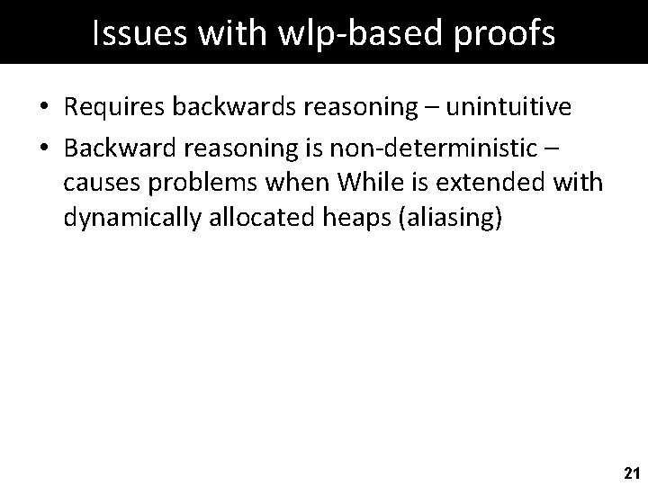
Strongest postcondition rules 1. 2. 3. 4. sp(skip, P) = P sp(x : = a, P) = � v. x=a[v/x] �P[v/x] sp(S 1; S 2, P) = sp(S 2, sp(S 1, P)) sp(if b then S 1 else S 2, P) = sp(S 1, b �P) �sp(S 2, � b �P) 5. sp(while b do {� } S, P) = ��� b where {b �� } S {� } and P � b �� 23
![Floyds strongest postcondition rule v xavx Pvx ass Floyd P x Floyd’s strongest postcondition rule v. x=a[v/x] �P[v/x] } [ass. Floyd] { P } x](https://slidetodoc.com/presentation_image_h2/857375281c873d7f27968f9d1e595abc/image-24.jpg)
Floyd’s strongest postcondition rule v. x=a[v/x] �P[v/x] } [ass. Floyd] { P } x : = a { � where v is a fresh variable The value of x in the pre-state • Example { z=x } x: =x+1 { ? } 24
![Floyds strongest postcondition rule v xavx Pvx ass Floyd P x Floyd’s strongest postcondition rule v. x=a[v/x] �P[v/x] } [ass. Floyd] { P } x](https://slidetodoc.com/presentation_image_h2/857375281c873d7f27968f9d1e595abc/image-25.jpg)
Floyd’s strongest postcondition rule v. x=a[v/x] �P[v/x] } [ass. Floyd] { P } x : = a { � where v is a fresh variable meaning: {x=z+1} • Example { z=x } x: =x+1 { � v. x=v+1 �z=v } • This rule is often considered problematic because it introduces a quantifier – needs to be eliminated further on • We will soon see a variant of this rule 25

exercise 26

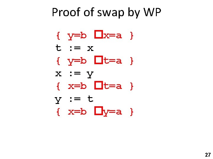
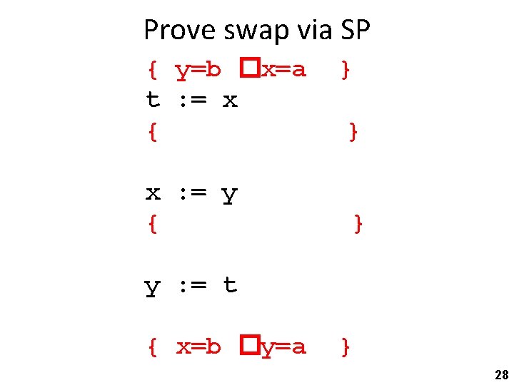
Proof of swap by WP { t { x { y=b �x=a : = x y=b �t=a : = y x=b �t=a : = t x=b �y=a } } 27

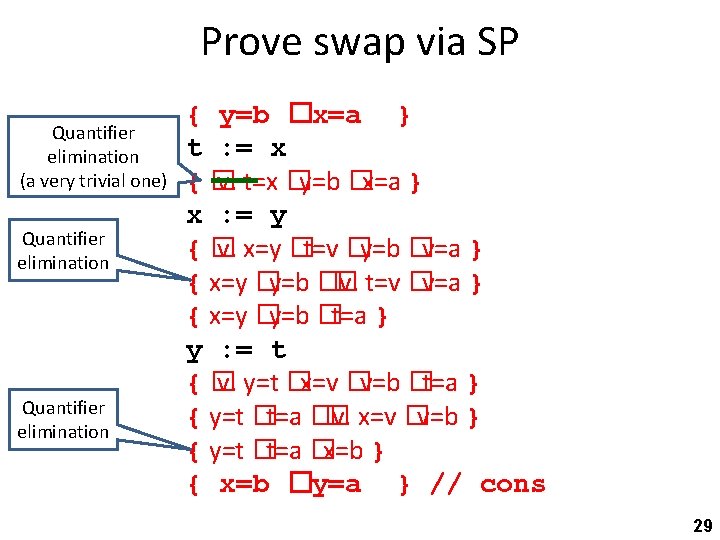
Prove swap via SP { y=b �x=a t : = x { x : = y { } } } y : = t { x=b �y=a } 28

Prove swap via SP Quantifier elimination (a very trivial one) Quantifier elimination { y=b �x=a } t : = x {� v. t=x �y=b �x=a } x : = y {� v. x=y �t=v �y=b �v=a } { x=y �y=b �� v. t=v �v=a } { x=y �y=b �t=a } y : = t {� v. y=t �x=v �v=b �t=a } { y=t �t=a �� v. x=v �v=b } { y=t �t=a �x=b } { x=b �y=a } // cons 29

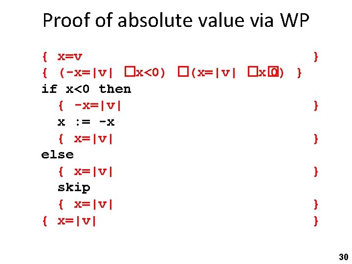
Proof of absolute value via WP { x=v } { (-x=|v| �x<0) �(x=|v| �x� 0) } if x<0 then { -x=|v| } x : = -x { x=|v| } else { x=|v| } skip { x=|v| } 30

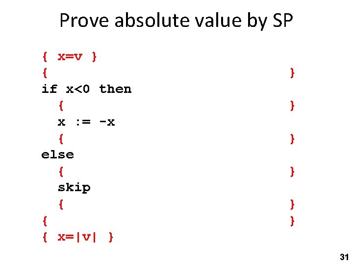
Prove absolute value by SP { x=v } { if x<0 then { x : = -x { else { skip { { { x=|v| } } } } 31

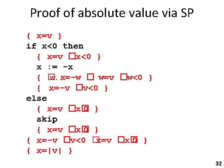
Proof of absolute value via SP { x=v } if x<0 then { x=v �x<0 } x : = -x { � w. x=-w � w=v �w<0 } { x=-v �v<0 } else { x=v �x� 0 } skip { x=v �x� 0 } { x=-v �v<0 �x=v �x� 0 } { x=|v| } 32

Making the proof system more practical 33
![Conjunction rule PSQ P S Q conjp P P Conjunction rule {P}S{Q} { P’ } S { Q’ } [conjp] { P �P’](https://slidetodoc.com/presentation_image_h2/857375281c873d7f27968f9d1e595abc/image-34.jpg)
Conjunction rule {P}S{Q} { P’ } S { Q’ } [conjp] { P �P’ } S {Q �Q’ } • Allows breaking up proofs into smaller, easier to manage, sub-proofs 34
![More useful rules PCQ P C Q disjp P More useful rules {P}C{Q} { P’ } C { Q’ } [disjp] { P](https://slidetodoc.com/presentation_image_h2/857375281c873d7f27968f9d1e595abc/image-35.jpg)
More useful rules {P}C{Q} { P’ } C { Q’ } [disjp] { P �P’ } C {Q �Q’ } {P}C{Q} [existp] v� FV(C) {� v. P } C { � v. Q } {P}C{Q} v� FV(C) [univp] {� v. P } C {� v. Q } [Invp] { F } C { F } Mod(C) �FV(F)={} • Mod(C) = set of variables assigned to in sub-statements of C • FV(F) = free variables of F 35
![Invariance Conjunction Constancy PCQ constancyp F P C F Invariance + Conjunction = Constancy {P}C{Q} [constancyp] { F �P } C { F](https://slidetodoc.com/presentation_image_h2/857375281c873d7f27968f9d1e595abc/image-36.jpg)
Invariance + Conjunction = Constancy {P}C{Q} [constancyp] { F �P } C { F �Q } Mod(C) �FV(F)={} • Mod(C) = set of variables assigned to in sub-statements of C • FV(F) = free variables of F 36

Strongest postcondition calculus practice By Vadim Plessky (http: //svgicons. sourceforge. net/) [see page for license], via Wikimedia Commons 37

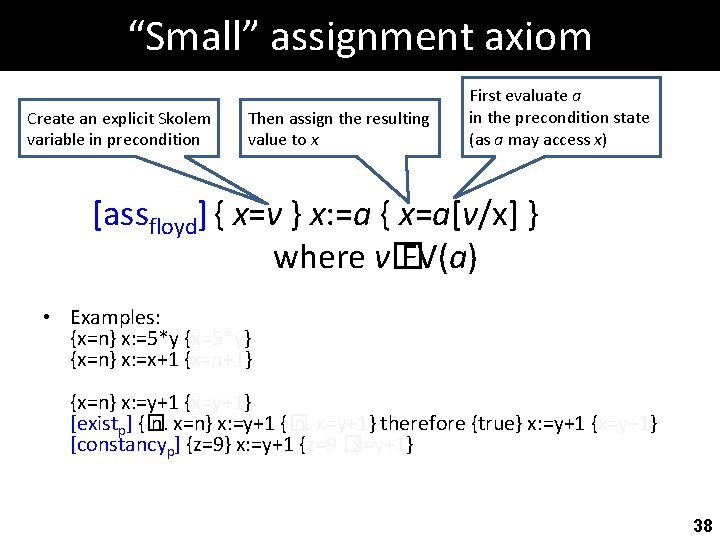
“Small” assignment axiom Create an explicit Skolem variable in precondition Then assign the resulting value to x First evaluate a in the precondition state (as a may access x) [assfloyd] { x=v } x: =a { x=a[v/x] } where v� FV(a) • Examples: {x=n} x: =5*y {x=5*y} {x=n} x: =x+1 {x=n+1} {x=n} x: =y+1 {x=y+1} [existp] {� n. x=n} x: =y+1 {� n. x=y+1} therefore {true} x: =y+1 {x=y+1} [constancyp] {z=9} x: =y+1 {z=9 �x=y+1} 38
![Small assignment axiom assfloyd xv x a xavx where v “Small” assignment axiom [assfloyd] { x=v } x: =a { x=a[v/x] } where v�](https://slidetodoc.com/presentation_image_h2/857375281c873d7f27968f9d1e595abc/image-39.jpg)
“Small” assignment axiom [assfloyd] { x=v } x: =a { x=a[v/x] } where v� FV(a) • Examples: {x=n} x: =5*y {x=5*y} {x=n} x: =x+1 {x=n+1} {x=n} x: =y+1 {x=y+1} [existp] {� n. x=n} x: =y+1 {� n. x=y+1} therefore {true} x: =y+1 {x=y+1} [constancyp] {z=9} x: =y+1 {z=9 �x=y+1} 39
![Small assignment axiom assfloyd xv x a xavx where v “Small” assignment axiom [assfloyd] { x=v } x: =a { x=a[v/x] } where v�](https://slidetodoc.com/presentation_image_h2/857375281c873d7f27968f9d1e595abc/image-40.jpg)
“Small” assignment axiom [assfloyd] { x=v } x: =a { x=a[v/x] } where v� FV(a) • Examples: {x=n} x: =5*y {x=5*y} {x=n} x: =x+1 {x=n+1} {x=n} x: =y+1 {x=y+1} [existp] {� n. x=n} x: =y+1 {� n. x=y+1} therefore {true} x: =y+1 {x=y+1} [constancyp] {z=9} x: =y+1 {z=9 �x=y+1} 40
![Small assignment axiom assfloyd xv x a xavx where v “Small” assignment axiom [assfloyd] { x=v } x: =a { x=a[v/x] } where v�](https://slidetodoc.com/presentation_image_h2/857375281c873d7f27968f9d1e595abc/image-41.jpg)
“Small” assignment axiom [assfloyd] { x=v } x: =a { x=a[v/x] } where v� FV(a) • Examples: {x=n} x: =5*y {x=5*y} {x=n} x: =x+1 {x=n+1} {x=n} x: =y+1 {x=y+1} [existp] {� n. x=n} x: =y+1 {� n. x=y+1} therefore {true} x: =y+1 {x=y+1} [constancyp] {z=9} x: =y+1 {z=9 �x=y+1} 41

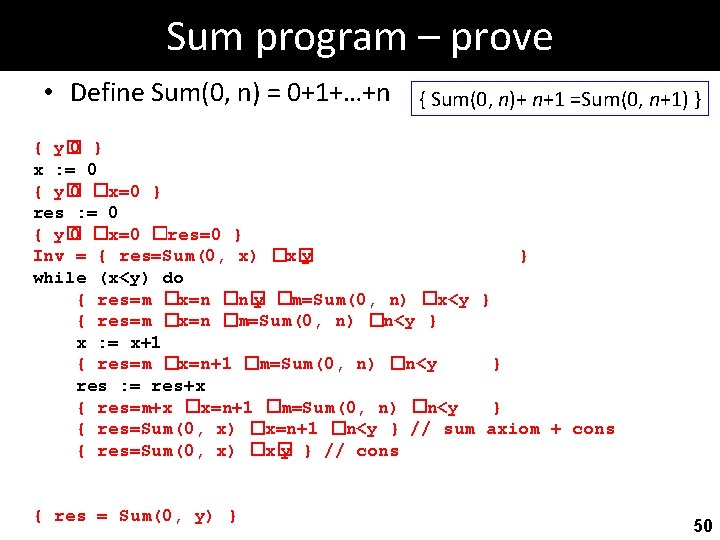
Sum program – specify • Define Sum(0, n) = 0+1+…+n { ? x : = 0 res : = 0 while (x<y) do x : = x+1 res : = res+x { ? } { Sum(0, n)+ n+1 =Sum(0, n+1) } Background axiom } 42

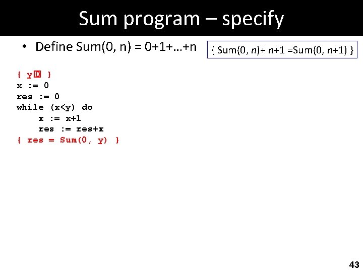
Sum program – specify • Define Sum(0, n) = 0+1+…+n { Sum(0, n)+ n+1 =Sum(0, n+1) } { y� 0 } x : = 0 res : = 0 while (x<y) do x : = x+1 res : = res+x { res = Sum(0, y) } 43

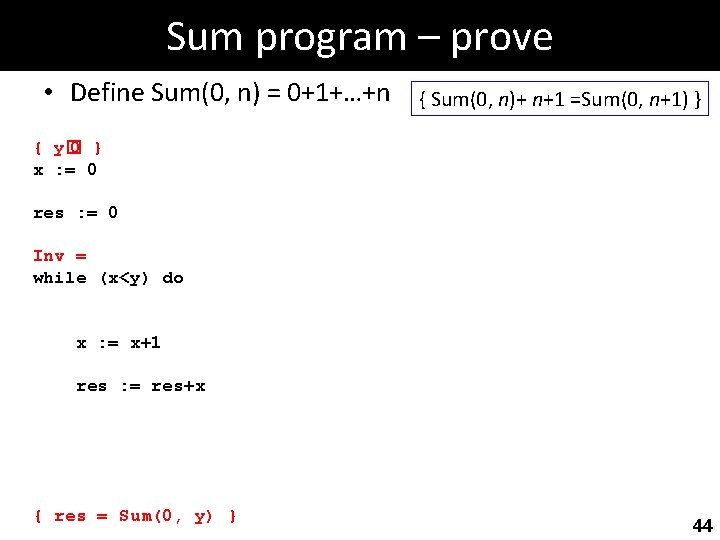
Sum program – prove • Define Sum(0, n) = 0+1+…+n { Sum(0, n)+ n+1 =Sum(0, n+1) } { y� 0 } x : = 0 res : = 0 Inv = while (x<y) do x : = x+1 res : = res+x { res = Sum(0, y) } 44

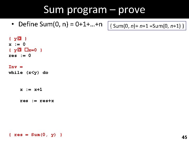
Sum program – prove • Define Sum(0, n) = 0+1+…+n { Sum(0, n)+ n+1 =Sum(0, n+1) } { y� 0 } x : = 0 { y� 0 �x=0 } res : = 0 Inv = while (x<y) do x : = x+1 res : = res+x { res = Sum(0, y) } 45

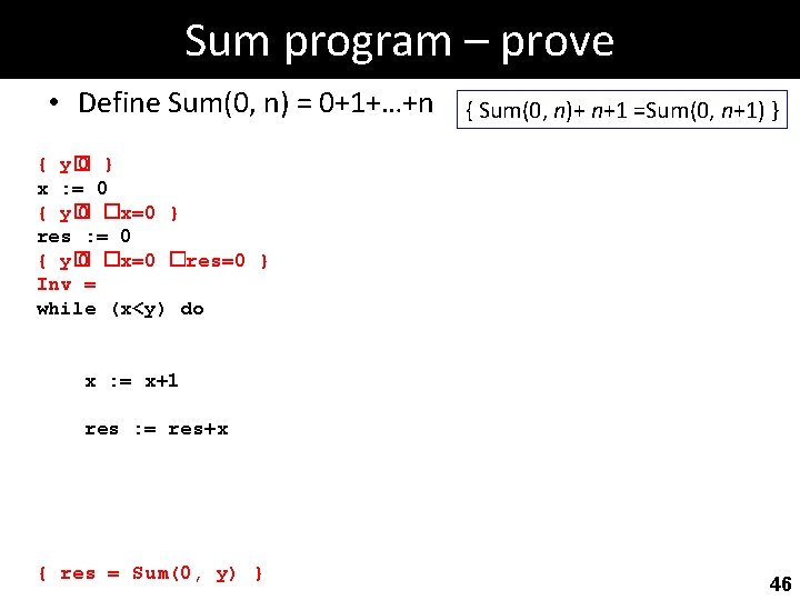
Sum program – prove • Define Sum(0, n) = 0+1+…+n { Sum(0, n)+ n+1 =Sum(0, n+1) } { y� 0 } x : = 0 { y� 0 �x=0 } res : = 0 { y� 0 �x=0 �res=0 } Inv = while (x<y) do x : = x+1 res : = res+x { res = Sum(0, y) } 46

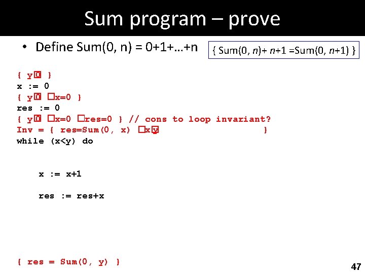
Sum program – prove • Define Sum(0, n) = 0+1+…+n { Sum(0, n)+ n+1 =Sum(0, n+1) } { y� 0 } x : = 0 { y� 0 �x=0 } res : = 0 { y� 0 �x=0 �res=0 } // cons to loop invariant? Inv = { res=Sum(0, x) �x� y } while (x<y) do x : = x+1 res : = res+x { res = Sum(0, y) } 47

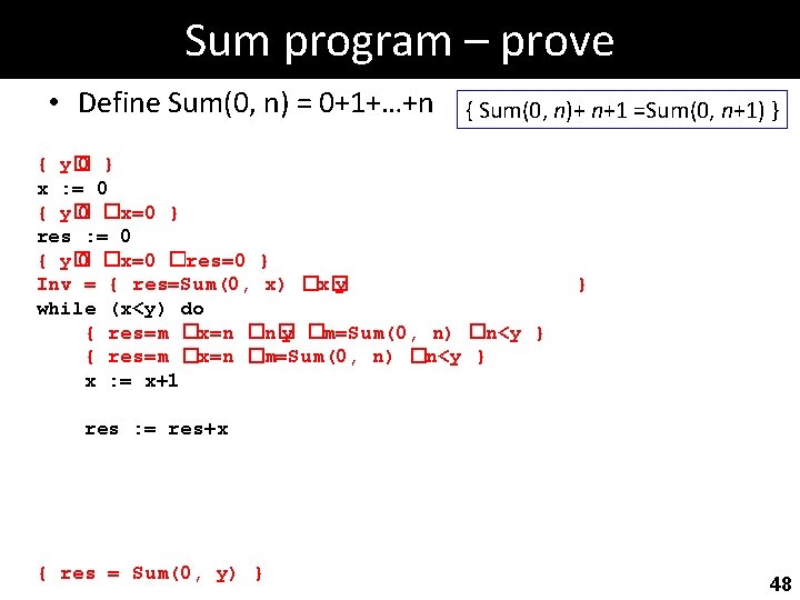
Sum program – prove • Define Sum(0, n) = 0+1+…+n { Sum(0, n)+ n+1 =Sum(0, n+1) } { y� 0 } x : = 0 { y� 0 �x=0 } res : = 0 { y� 0 �x=0 �res=0 } Inv = { res=Sum(0, x) �x� y while (x<y) do { res=m �x=n �n� y �m=Sum(0, n) �n<y } { res=m �x=n �m=Sum(0, n) �n<y } x : = x+1 } res : = res+x { res = Sum(0, y) } 48

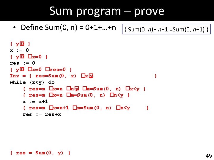
Sum program – prove • Define Sum(0, n) = 0+1+…+n { Sum(0, n)+ n+1 =Sum(0, n+1) } { y� 0 } x : = 0 { y� 0 �x=0 } res : = 0 { y� 0 �x=0 �res=0 } Inv = { res=Sum(0, x) �x� y } while (x<y) do { res=m �x=n �n� y �m=Sum(0, n) �x<y } { res=m �x=n �m=Sum(0, n) �n<y } x : = x+1 { res=m �x=n+1 �m=Sum(0, n) �n<y } res : = res+x { res = Sum(0, y) } 49

Sum program – prove • Define Sum(0, n) = 0+1+…+n { Sum(0, n)+ n+1 =Sum(0, n+1) } { y� 0 } x : = 0 { y� 0 �x=0 } res : = 0 { y� 0 �x=0 �res=0 } Inv = { res=Sum(0, x) �x� y } while (x<y) do { res=m �x=n �n� y �m=Sum(0, n) �x<y } { res=m �x=n �m=Sum(0, n) �n<y } x : = x+1 { res=m �x=n+1 �m=Sum(0, n) �n<y } res : = res+x { res=m+x �x=n+1 �m=Sum(0, n) �n<y } { res=Sum(0, x) �x=n+1 �n<y } // sum axiom + cons { res=Sum(0, x) �x� y } // cons { res = Sum(0, y) } 50

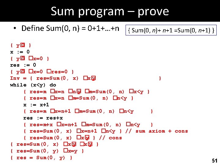
Sum program – prove • Define Sum(0, n) = 0+1+…+n { Sum(0, n)+ n+1 =Sum(0, n+1) } { y� 0 } x : = 0 { y� 0 �x=0 } res : = 0 { y� 0 �x=0 �res=0 } Inv = { res=Sum(0, x) �x� y } while (x<y) do { res=m �x=n �n� y �m=Sum(0, n) �x<y } { res=m �x=n �m=Sum(0, n) �n<y } x : = x+1 { res=m �x=n+1 �m=Sum(0, n) �n<y } res : = res+x { res=m+x �x=n+1 �m=Sum(0, n) �n<y } { res=Sum(0, x) �x=n+1 �n<y } // sum axiom + cons { res=Sum(0, x) �x� y } // cons { res=Sum(0, x) �x� y } { res=Sum(0, y) �x=y } { res = Sum(0, y) } 51

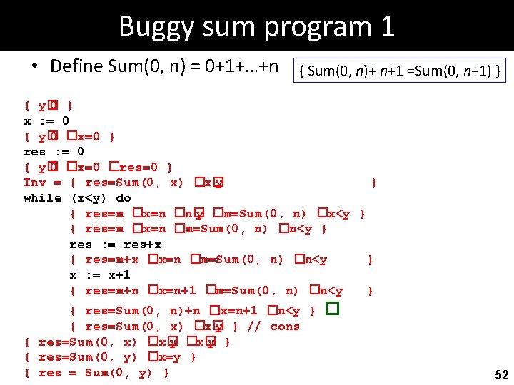
Buggy sum program 1 • Define Sum(0, n) = 0+1+…+n { Sum(0, n)+ n+1 =Sum(0, n+1) } { y� 0 } x : = 0 { y� 0 �x=0 } res : = 0 { y� 0 �x=0 �res=0 } Inv = { res=Sum(0, x) �x� y } while (x<y) do { res=m �x=n �n� y �m=Sum(0, n) �x<y } { res=m �x=n �m=Sum(0, n) �n<y } res : = res+x { res=m+x �x=n �m=Sum(0, n) �n<y } x : = x+1 { res=m+n �x=n+1 �m=Sum(0, n) �n<y } { res=Sum(0, n)+n �x=n+1 �n<y } { res=Sum(0, x) �x� y } // cons { res=Sum(0, x) �x� y } { res=Sum(0, y) �x=y } { res = Sum(0, y) } � 52

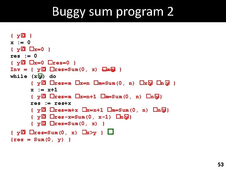
Buggy sum program 2 { y� 0 } x : = 0 { y� 0 �x=0 } res : = 0 { y� 0 �x=0 �res=0 } Inv = { y� 0 �res=Sum(0, x) �x� y } while (x� y) do { y� 0 �res=m �x=n �m=Sum(0, n) �x� y �n� y } x : = x+1 { y� 0 �res=m �x=n+1 �m=Sum(0, n) �n� y} res : = res+x { y� 0 �res=m+x �x=n+1 �m=Sum(0, n) �n� y} { y� 0 �res-x=Sum(0, x-1) �n� y} { y� 0 �res=Sum(0, x) �x>y } {res = Sum(0, y) } � 53

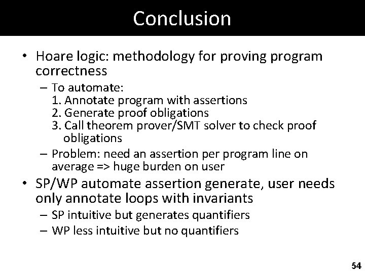
Conclusion • Hoare logic: methodology for proving program correctness – To automate: 1. Annotate program with assertions 2. Generate proof obligations 3. Call theorem prover/SMT solver to check proof obligations – Problem: need an assertion per program line on average => huge burden on user • SP/WP automate assertion generate, user needs only annotate loops with invariants – SP intuitive but generates quantifiers – WP less intuitive but no quantifiers 54

see you next time 55