SpreadsheetBased Decision Support Systems Chapter 8 The Solver

Spreadsheet-Based Decision Support Systems Chapter 8: The Solver and Mathematical Programming Prof. Name Position University Name name@email. com (123) 456 -7890
Overview v v v Introduction Formulating Mathematical Programs The Excel Solver Applications of the Solver Summary 2
Introduction v Formulating a mathematical program by determining its decision variables, constraints, and objective function v The difference between linear, integer, and nonlinear programming problems v Using the Excel Solver to solve a mathematical program v Preparing the spreadsheet with the model parts and then enter the corresponding cells into the Solver window v Reading the Solver reports v Example linear, integer, and nonlinear programming problems 3
Formulating Mathematical Programs v Parts of the Mathematical Program v Linear, Integer, and Nonlinear Programming 4
Parts of the Mathematical Program v Decision Variables = variables assigned to a quantity or response that must be determined in the problem v Objective Function = equation which states the goal of the model – Maximize – Minimize v Constraints = equations which state limitations of the problem v To solve the model, each constraint must be considered simultaneously in conjunction with the objective function 5
Linear Integer and Nonlinear Programming v Linear Programming problem = there is a linear relationship among all constraints and the objective function v Integer Programming problem = decision variables can only take integer values in a given range (these integer values can also be boolean = 0 or 1 only) v Nonlinear Programming problem = do not have a linear objective function and/or constraints. NLP problems must use more challenging methods to solve these complex equations. 6
The Excel Solver v The Solver Steps v Understanding Solver Reports 7
The Solver Steps v Step 1: Read and Interpret the Problem – Step 1. 1: determine the decision variables – Step 1. 2: state the objective function – Step 1. 3: state any constraints v Step 2: Prepare the Spreadsheet – Step 2. 1: Enter the decision variables – Step 2. 2: Enter the constraints – Step 2. 3: Enter the objective function v Step 3: Solve the model with the Solver – – – Step 3. 1: Set the Target Cell and choose Min or Max Step 3. 2: Select Changing Cells Step 3. 3: Add Constraints Step 3. 4: Set Solver Options Step 3. 5: Solve and review Results 8
Product Mix Problem v A company produces six different types of products. They want to schedule their production to determine how much of each product type should be produced in order to maximize their profits. This is known as the Product Mix problem. v Production of each product type requires labor and raw materials; but the company is limited by the amount of resources available. v There is also a limited demand for each product, and no more than this demand per product type can be produced. Input tables for the necessary resources and the demand are given. 9
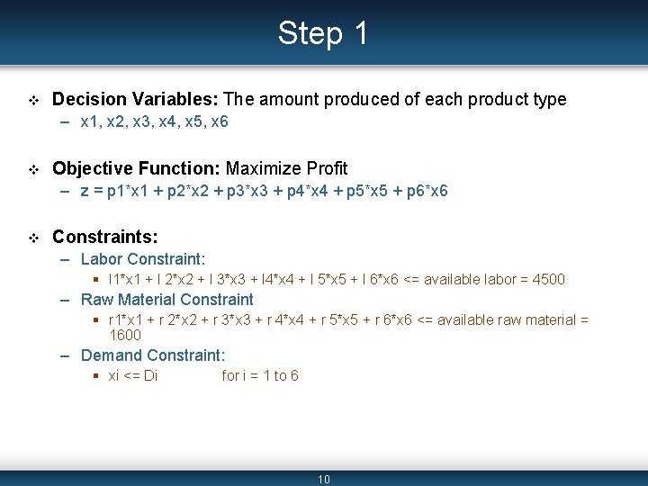
Step 1 v Decision Variables: The amount produced of each product type – x 1, x 2, x 3, x 4, x 5, x 6 v Objective Function: Maximize Profit – z = p 1*x 1 + p 2*x 2 + p 3*x 3 + p 4*x 4 + p 5*x 5 + p 6*x 6 v Constraints: – Labor Constraint: § l 1*x 1 + l 2*x 2 + l 3*x 3 + l 4*x 4 + l 5*x 5 + l 6*x 6 <= available labor = 4500 – Raw Material Constraint § r 1*x 1 + r 2*x 2 + r 3*x 3 + r 4*x 4 + r 5*x 5 + r 6*x 6 <= available raw material = 1600 – Demand Constraint: § xi <= Di for i = 1 to 6 10
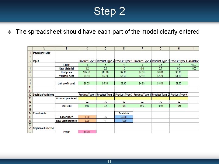
Step 2 v The spreadsheet should have each part of the model clearly entered 11
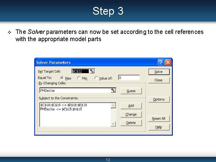
Step 3 v The Solver parameters can now be set according to the cell references with the appropriate model parts 12
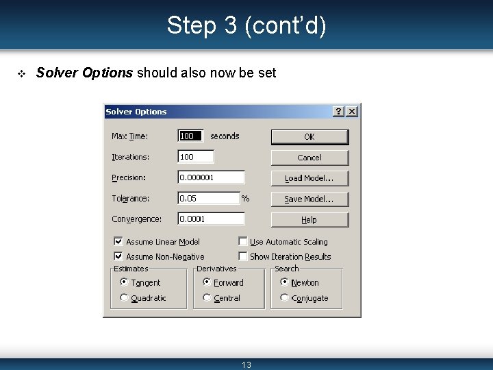
Step 3 (cont’d) v Solver Options should also now be set 13
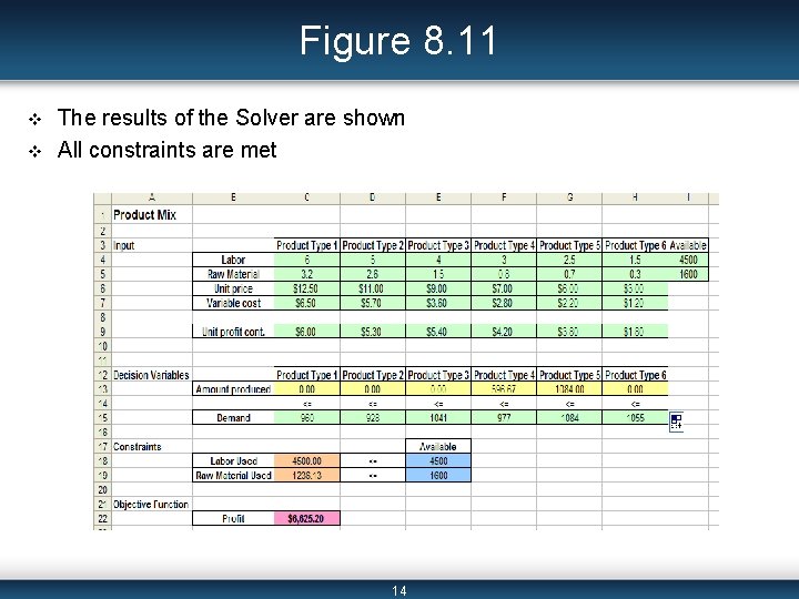
Figure 8. 11 v v The results of the Solver are shown All constraints are met 14
Solver Reports v Answer Report = lists the target cell and the changing cells with their original and final values, constraints, and information about the constraints. v Sensitivity Report = shows how sensitive the solution is to small changes in the objective function formula or the constraints. v Limits Report = lists the target cell and the changing cells with their respective values, lower and upper limits, and target values. 15
Applications of the Solver v Transportation Problem v Workforce Scheduling v Capital Budgeting v Warehouse Location 16
Transportation Problem v A company ships their products from three different plants (one in LA, one in Atlanta, and one in New York City) to four regions of the United States (East, Midwest, South, West). v Each plant has a capacity on how many products can be sent out, and each region has a demand of products they must receive. v There is a different transportation cost between each plant, or each city, and each region. v The company wants to determine how many products each plant should ship to each region in order to minimize the total transportation cost. 17
Transportation Problem (cont’d) v Decision variables: – The amount to ship from each plant to each region v Constraints : – Demand: the total number of products received by a region (from each plant) is greater than or equal to its demand – Capacity: the total number of products shipped from a plant (to each region) is less than or equal to its capacity v Objective function: – Minimize the total transportation costs 18
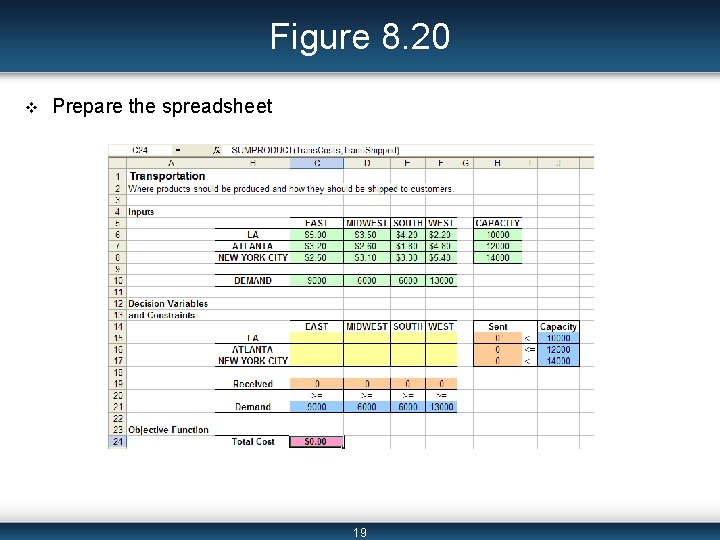
Figure 8. 20 v Prepare the spreadsheet 19
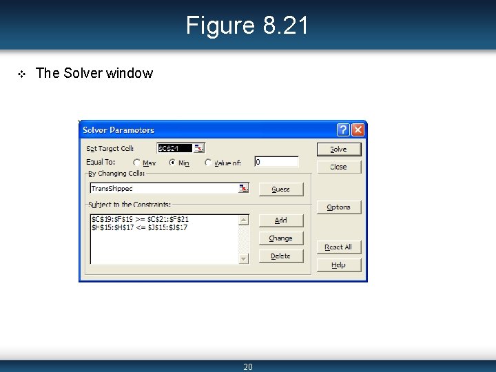
Figure 8. 21 v The Solver window 20
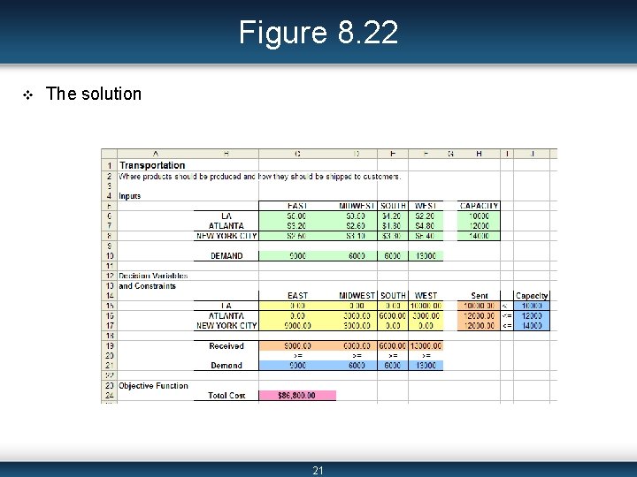
Figure 8. 22 v The solution 21
Workforce Scheduling v A company wants to schedule its employees for every day of the week. v Employees work 5 days consecutively, so the company wants to schedule on which day each employee starts working; that is how many employees start working each day. v There is a certain number of employees needed each day of the week. v The objective function is to find the schedule which minimizes the total number of employees working for the week. 22
Workforce Scheduling (cont’d) v Decision variables: – The number of employees that will begin working (for 5 consecutive days) on each day of the week v Constraints: – The total number of employees working on a given day (regardless of which day they started working) is greater than or equal to the number of employees needed on that particular day v objective function – Minimize the total number of employees needed 23
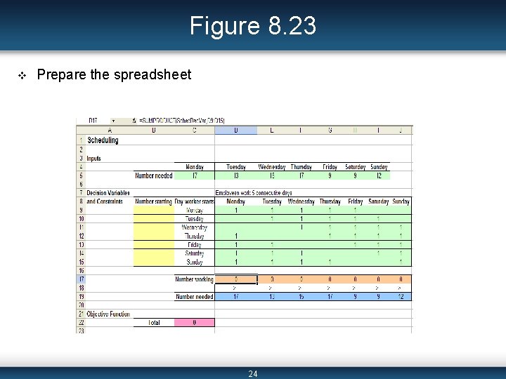
Figure 8. 23 v Prepare the spreadsheet 24
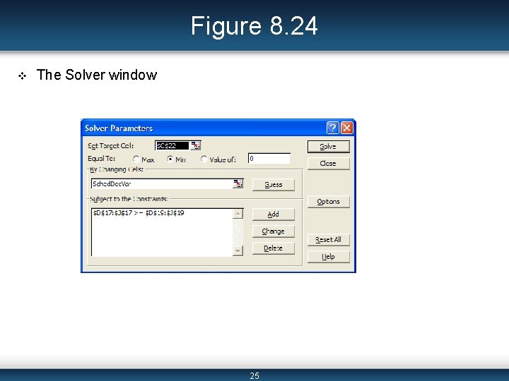
Figure 8. 24 v The Solver window 25
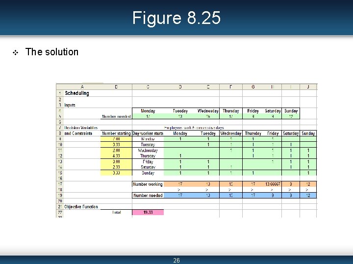
Figure 8. 25 v The solution 26
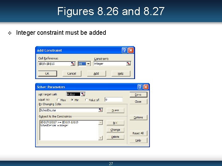
Figures 8. 26 and 8. 27 v Integer constraint must be added 27
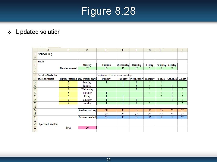
Figure 8. 28 v Updated solution 28
Capital Budgeting v There are 20 projects that a company, or individual, can invest in. v Each project has a net present value (NPV) and cost per year given. v The company, or investor, wants to determine how much to invest in each project, given a limited amount of yearly funds available, in order to maximize the total NPV of the investment. 29
Capital Budgeting (cont’d) v Decision variables: – Which projects we do and do not invest in v Constraints: – No more than the yearly available funds can be spent each year v Objective Function: – Maximize the total NPV 30
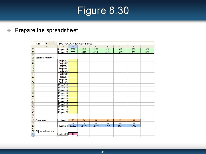
Figure 8. 30 v Prepare the spreadsheet 31
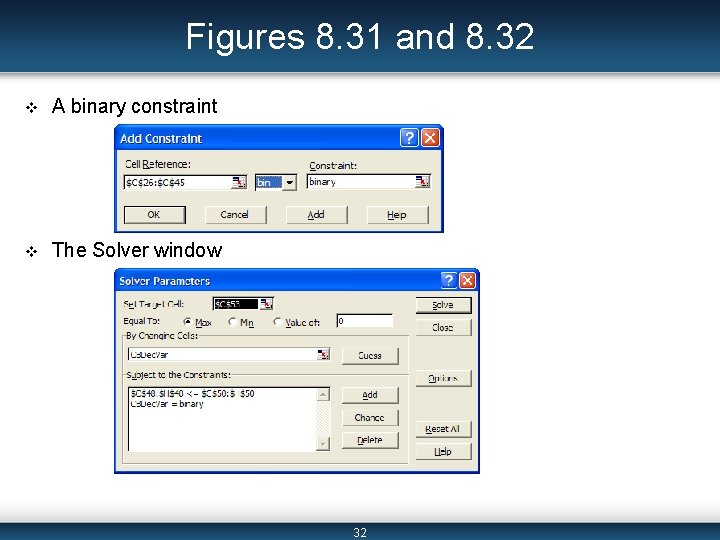
Figures 8. 31 and 8. 32 v A binary constraint v The Solver window 32
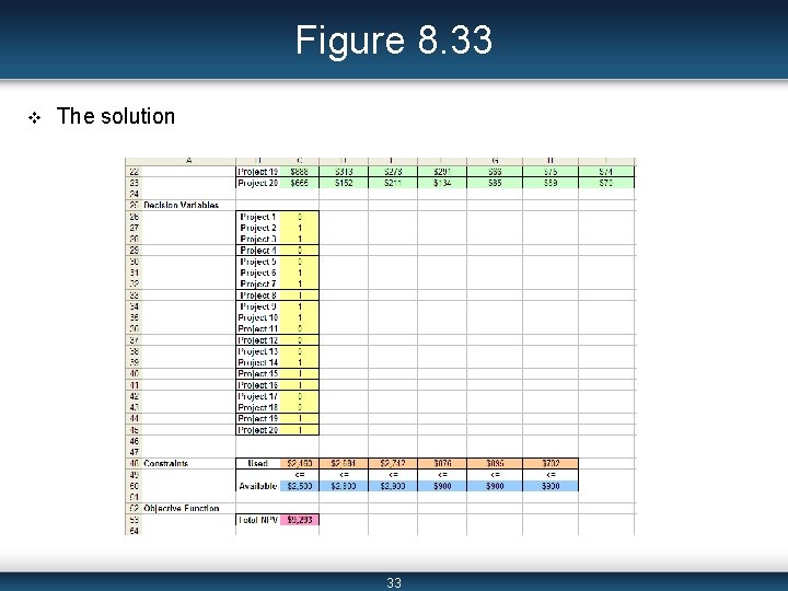
Figure 8. 33 v The solution 33
Warehouse Location v A company stores all of its products in one warehouse. v It has customers in cities around the United States and is trying to determine the best location of their warehouse in order to minimize the total transportations costs. v Each city’s location is given by its latitude and longitude. The number of shipments made to each city is also given. We are to determine the warehouse location based on its latitude and longitude values. 34
Warehouse Location (cont’d) v Decision variable: – The latitude and longitude values of the location of the warehouse v Constraints: – The latitude and longitude for the warehouse location must be between the values of 0 and 120 v Objective function: – Minimize the total distance traveled from the warehouse to each city 35
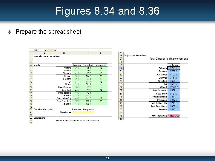
Figures 8. 34 and 8. 36 v Prepare the spreadsheet 36
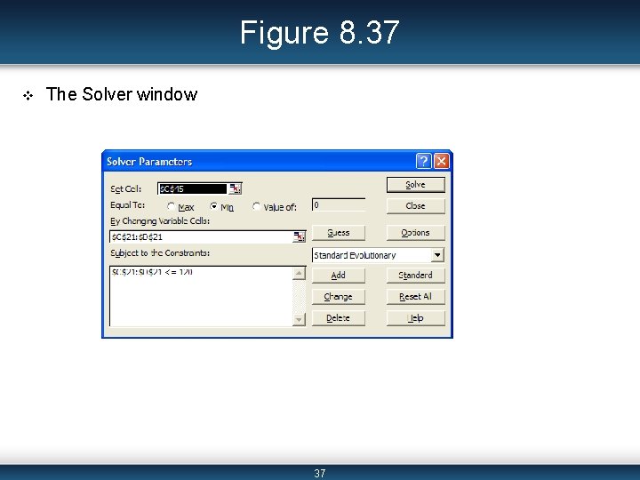
Figure 8. 37 v The Solver window 37
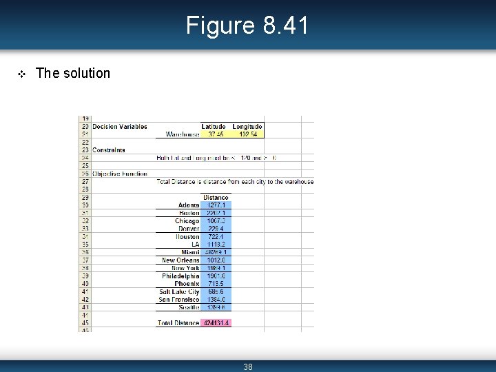
Figure 8. 41 v The solution 38
Summary v The three parts of a mathematical model are decision variables, objective function, and constraints. v The three primary types of mathematical models are linear, integer, and nonlinear programming problems. v Using Solver involves three main steps: reading and interpreting the problem to determine three parts of the model; preparing the spreadsheet so that Solver can read the data; and running the Solver. v LP examples are Transportation and Workforce Scheduling. An IP example is Capital Budgeting, and an NLP example is the Warehouse Location problem. – We use the Premium Solver to solve NLP problems since the Genetic Algorithm is more accurate. 39
Additional Links v (place links here) 40
- Slides: 40