Spots Ray Fan Optical Path Difference OPD Point

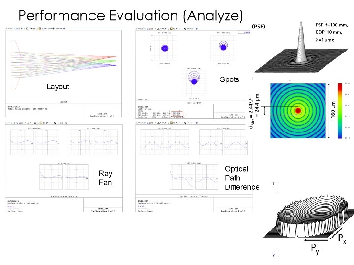
Spots, Ray Fan, Optical Path Difference (OPD), Point Spread Function (PSF)

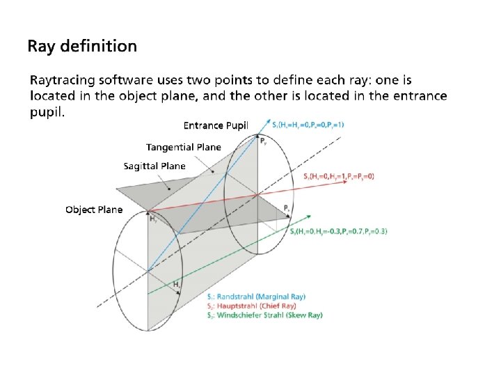
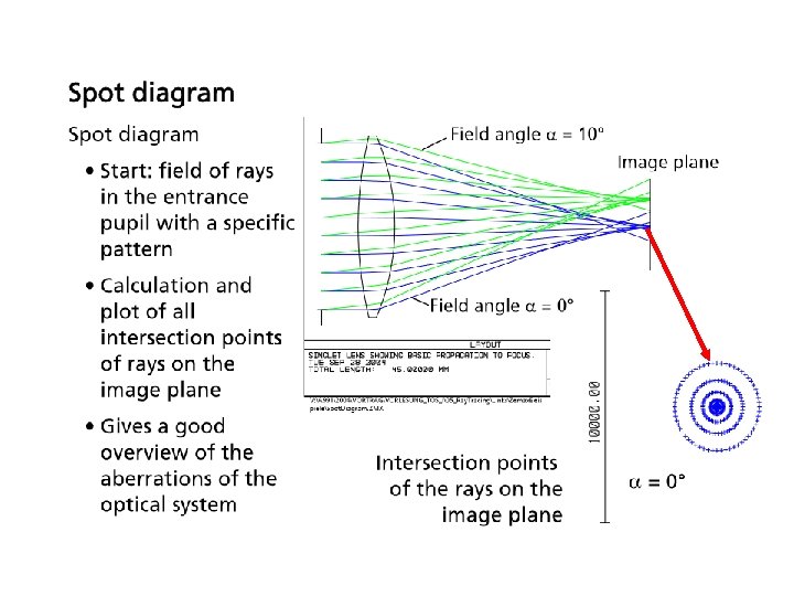
What is a Point Spread Function • The PSF of an optical system is the irradiance distribution that results from a single point source in object space. • A telescope forming an image of a distant star is a good example: the star is so far away that for all practical purposes it can be considered a point. • Although the source may be a point, the image is not. There are two main reasons. First, aberrations in the optical system will spread the image over a finite area. Second, diffraction effects will also spread the image, even in a system that has no aberrations. Zemax has three basic types of PSF calculations: a geometric (no diffraction) spot diagram, and the diffraction based FFT and Huygens PSF.

When to use the Spot Diagram, FFT PSF, and Huygens PSF • Use the spot diagram when: The geometric aberrations are large compared to the diffraction effects. This can be checked using the "Airy Disk" scale option on the spot diagram. • Use the FFT PSF when: The chief ray makes a small angle with respect to the image surface normal. • Use the Huygens PSF when: Maximum accuracy is desired.

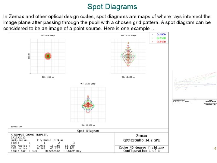
Spot Diagram • The sample optical system used here is a single parabolic F/5 mirror with a focal length of 50 mm. The object is at infinity. This system is a simplified Newtonian telescope, and the sample file is PSF_Newtonian. ZMX

Spot Diagram • Note the spot diagram is a collection of points, with each point representing a single ray. There is no interaction or interference between the rays. The spot diagram is very effective at showing the effects of the geometric, or ray aberrations. • The off axis geometric PSF clearly shows the coma and astigmatism of the system. On axis however, the spot diagram predicts perfect imagery. Is this an accurate representation of the optical system performance? To answer this question for the spot diagram results, we need to compare the spot distribution to the diffraction limited response. A quick way to compare the geometric aberrations to the diffraction limit is to add an Airy disk reference ellipse to the spot diagram. Open the settings box and change Show Scale to "Airy Disk":

Spot diagram and Airy disk

Example : Spot diagram and Airy disk

Spot diagram and Airy disk • On axis, the spot is much smaller than the Airy Disk, while off axis the spot is much larger than the Airy Disk. This indicates the spot diagram is a useful and reasonable indicator of performance off axis only. To compute a more accurate PSF both on and off axis, a consideration of diffraction will be required. Generally speaking, the spot diagram is useful if the aberrations are large compared to the diffraction limited performance of the system.

The FFT PSF • The Fast Fourier Transform (FFT) algorithm has been widely applied to frequency analysis of many electrical and optical systems. Conceptually, the FFT decomposes a spatial distribution into a frequency domain distribution. • There is also a summary of diffraction theory in the chapter "Physical Optics Propagation" in the Zemax manual, reference • Both of these references describe Fresnel and Fraunhofer diffraction theory.

The FFT PSF

The FFT PSF

1 3 2 4

The FFT PSF • Display is 128 x 128, Field is 2, Type is Logarithmic, and the Show As is set to False Color. Here is the resulting PSF:

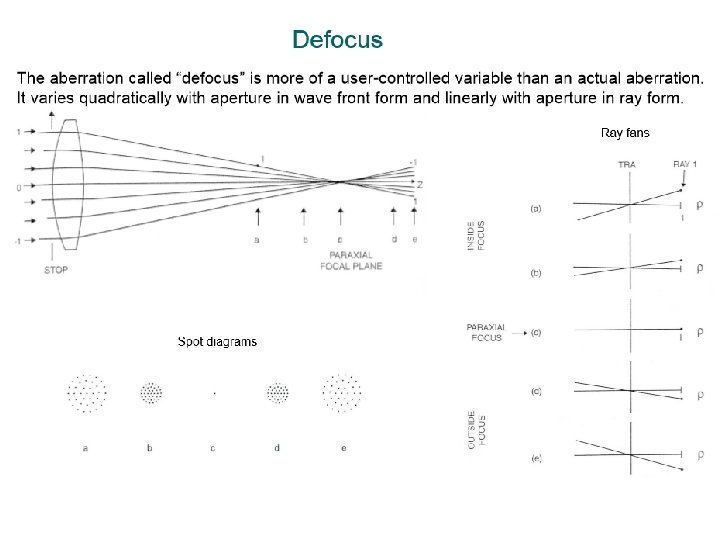
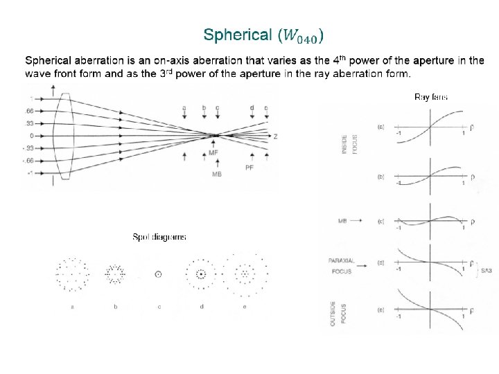
Ray fan • These curves can take several different forms , depending on the particular application of the optical system. The most common form is the transverse ray aberration curve. It is also called lateral aberration , or ray intercept curve (also referred to by the misleading term ‘‘rim ray plots’’). These plots are generated by tracing fans of rays from a specific object point for finite object distances (or a specific field angle for an object at infinity) to a linear array of points across the entrance pupil of the lens. The curves are plots of the ray error at an evaluation plane measured from the chief ray as a function of the relative ray height in the entrance pupil (Fig. 1). For a focal systems , one generally plots angular aberrations , the differences between the tangents of exiting rays and their chief ray in image space.

Relation between Ray Error and Wavefront Error TRA In a system with aberrations, rays from different positions in the exit pupil may miss the ideal image position by various amounts when they reach the image plane. This is known as “Transverse Ray Aberration”, or ‘TRA’. Zemax will plot a “ray fan” (Analysis – Fans – Ray Aberration): This is, for each field point, a plot of the TRA for rays that pass through different positions in the Exit Pupil. This plot is a slice through the pupil in the x-direction plotted against TRA in the x-direction, and a similar plot in the y-direction.

High Aberration Low Aberration Lens correction

Transverse Ray Fan

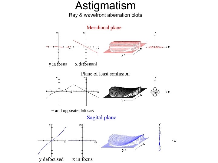
Tangential plane

CLC = circle of least confusion

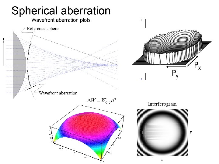
Optical Path Difference (OPD)

Wave Front

Wavefront and Ray Tracing Exit Pupil Stop Entrance Pupil Ideal Spherical Wavefront Ray trace programs will report “Wavefront Errors” at the Exit Pupil of a system.

Relation OPD, Wavefront, spot diagram

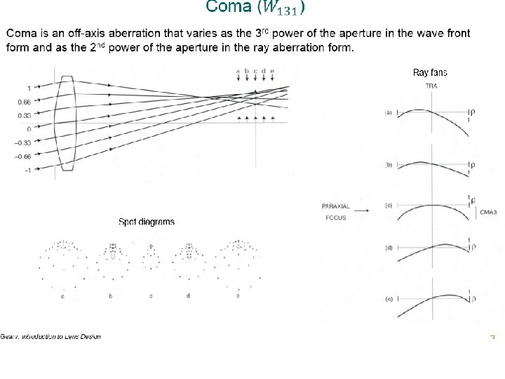
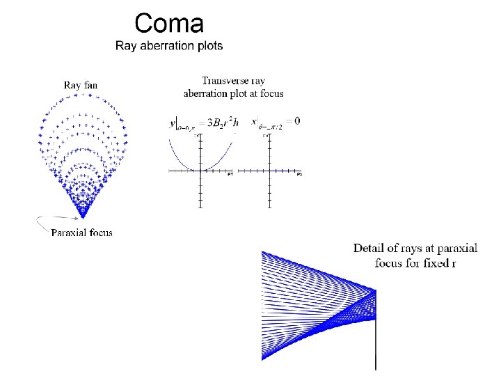
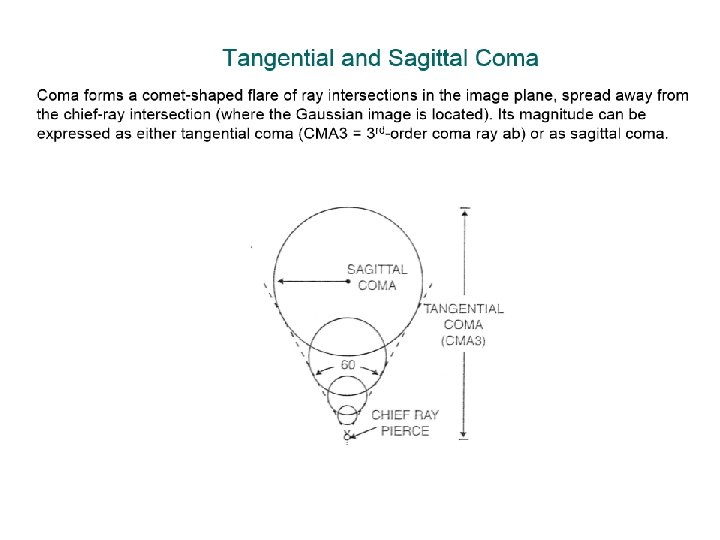
Coma • “Comet”-shaped spot • Chief ray is at apex of coma pattern • Centroid is shifted from chief ray! • Centroid shifts with change in focus! Wavefront

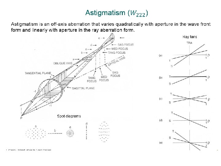
astigmatism

Wavefront Errors and Ray Tracing Exit Pupil Stop Entrance Pupil Ideal Spherical Wavefront Actual, Abberrated Wavefront Ray trace programs will report “Wavefront Errors” at the Exit Pupil of a system. The errors are the difference between the actual wavefront and the ideal spherical wavefront converging on the image point.

Zemax does not normally propagate waves through an optical system, but uses a geometric relationship between Ray errors and wavefront errors to calculate the wavefront error map: R Since rays are always perpendicular to wavefronts, a wavefront tilt error (at some location in the pupil) corresponds directly to a Transverse Ray error (TRA) at the image plane. The wavefront aberration, W, is the sag difference between the actual wavefront and the ideal spherical wavefront centered on the paraxial image point. The angle, a, between the ideal ray and the real ray is just slope of W, , and the Transverse Ray Aberration is: Note that, while this method accounts for wave aberrations at the exit pupil (and can, therefore, be used to derive some image aberrations) it takes no account of wave diffraction effects throughout the rest of the optical system, as a true wave propagation method would.

By tracing a number of rays through the pupil, and measuring the TRA of each, we can get the slope of W; then by numerical integration, we can find the wavefront aberrations, W. Somewhat remarkably, therefore, we can find W to a small fraction of a wavelength without having to track the path length of the rays we use to find it. (This is the way a Shack. Hartmann wavefront sensor works. ) A wavefront sensor can be used to measure the wavefront distortions introduced by an optical system. If you start with a diffraction limited point source (a light source focused through a small pinhole, say), the wave front sensor will measure the distortions of the collimated wave. Since the optics are reversable, this also gives the distortions present when light is focused by the system. Wavefront Dif. Lim Point Sensor Source

Measurements of wavefront distortion can be done by interferometry. This requires that the light used be coherent (e. g. , from a laser). A Shack. Hartmann wavefront sensor, however, can work in incoherent and even broad-band light: A Shack-Hartmann wavefront sensor consists of an array of micro-lenses focusing portions of an incoming wavefront onto position-sensitive detectors. The local tilt in the wavefront causes the focused spots to shift accordingly. Once an array of wavefront tilts has been calculated, numerical integration gives the wavefront shape.

Len data editor