Spooky Stuff in Metric Space Spooky Stuff Data

Spooky Stuff in Metric Space

Spooky Stuff Data Mining in Metric Space Rich Caruana Alex Niculescu Cornell University

Motivation #1

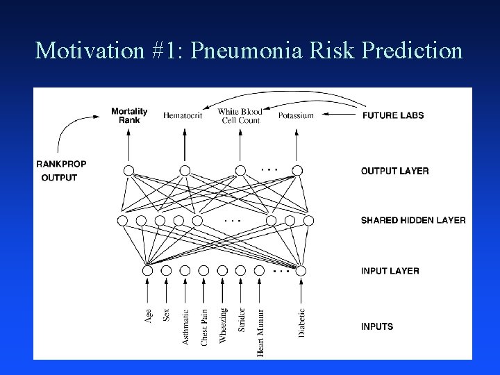
Motivation #1: Pneumonia Risk Prediction

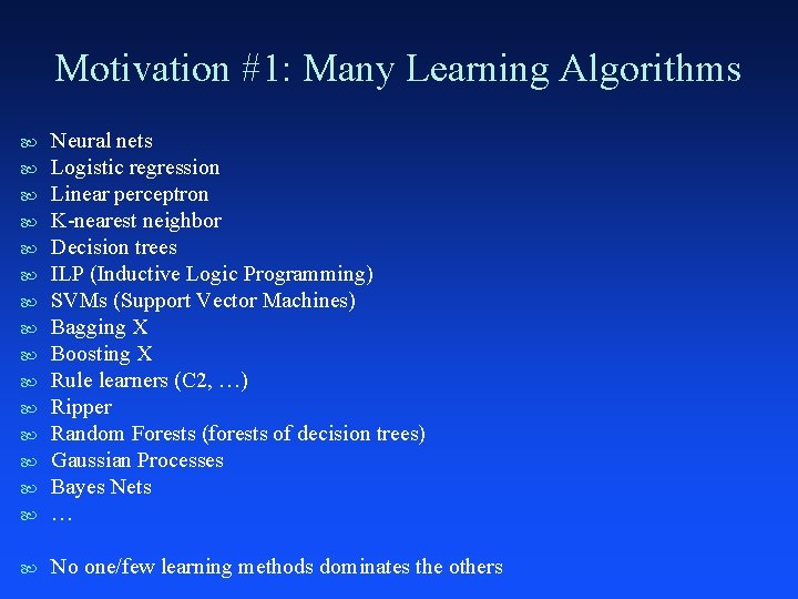
Motivation #1: Many Learning Algorithms Neural nets Logistic regression Linear perceptron K-nearest neighbor Decision trees ILP (Inductive Logic Programming) SVMs (Support Vector Machines) Bagging X Boosting X Rule learners (C 2, …) Ripper Random Forests (forests of decision trees) Gaussian Processes Bayes Nets … No one/few learning methods dominates the others

Motivation #2

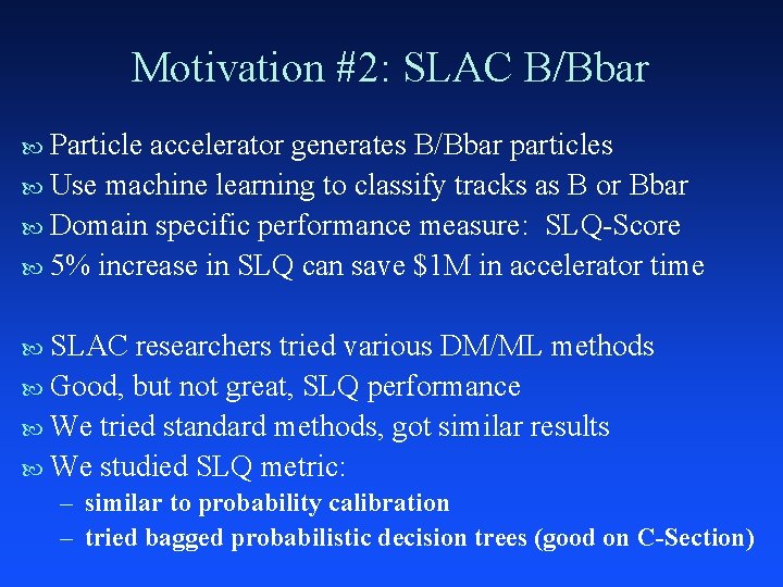
Motivation #2: SLAC B/Bbar Particle accelerator generates B/Bbar particles Use machine learning to classify tracks as B or Bbar Domain specific performance measure: SLQ-Score 5% increase in SLQ can save $1 M in accelerator time SLAC researchers tried various DM/ML methods Good, but not great, SLQ performance We tried standard methods, got similar results We studied SLQ metric: – similar to probability calibration – tried bagged probabilistic decision trees (good on C-Section)

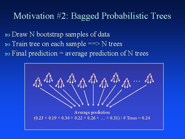
Motivation #2: Bagged Probabilistic Trees Draw N bootstrap samples of data Train tree on each sample ==> N trees Final prediction = average prediction of N trees … Average prediction (0. 23 + 0. 19 + 0. 34 + 0. 22 + 0. 26 + … + 0. 31) / # Trees = 0. 24

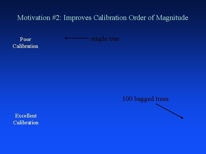
Motivation #2: Improves Calibration Order of Magnitude Poor Calibration single tree 100 bagged trees Excellent Calibration

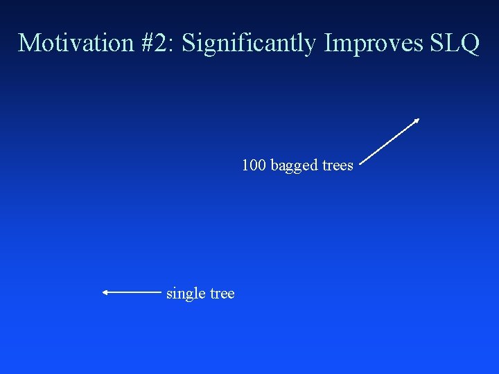
Motivation #2: Significantly Improves SLQ 100 bagged trees single tree

Motivation #2 Can we automate this analysis of performance metrics so that it’s easier to recognize which metrics are similar to each other?

Motivation #3

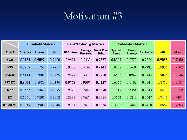
Motivation #3 Threshold Metrics Rank/Ordering Metrics Probability Metrics Average Break Even Precision Point Squared Error Cross. Entropy Calibration SAR Mean 0. 9621 0. 9335 0. 9377 0. 8767 0. 8778 0. 9824 0. 9055 0. 9156 0. 9487 0. 9552 0. 9167 0. 9142 0. 8532 0. 8634 0. 9881 0. 8956 0. 9102 0. 8609 0. 9465 0. 9674 0. 9416 0. 9220 0. 8588 0. 8942 0. 9744 0. 9036 0. 9086 0. 8904 0. 8986 0. 9574 0. 9778 0. 9597 0. 9427 0. 6066 0. 6107 0. 9241 0. 8710 0. 8631 KNN 0. 7557 0. 8463 0. 9095 0. 9370 0. 8847 0. 8890 0. 7612 0. 7354 0. 9843 0. 8470 0. 8559 DT 0. 5261 0. 7891 0. 8503 0. 8678 0. 7674 0. 7954 0. 5564 0. 6243 0. 9647 0. 7445 0. 7491 BST-STMP 0. 7319 0. 7903 0. 9046 0. 9187 0. 8610 0. 8336 0. 3038 0. 2861 0. 9410 0. 6589 0. 7303 Model Accuracy F-Score Lift ROC Area SVM 0. 8134 0. 9092 0. 9480 ANN 0. 8769 0. 8752 BAG-DT 0. 8114 BST-DT

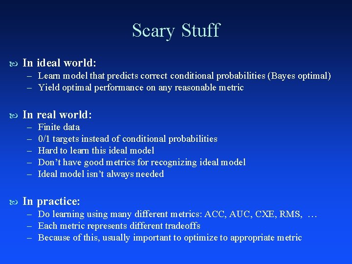
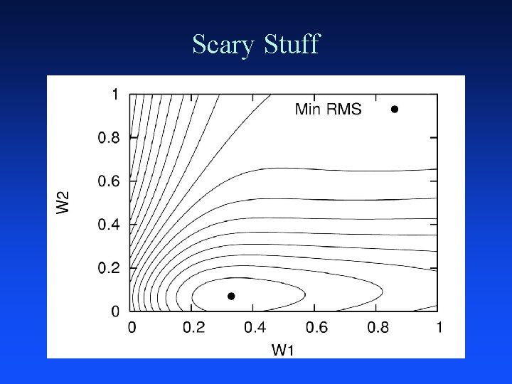
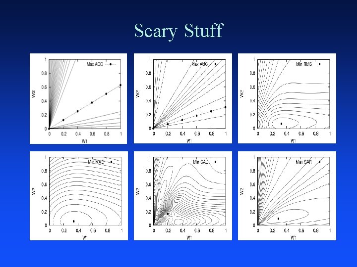
Scary Stuff In ideal world: – Learn model that predicts correct conditional probabilities (Bayes optimal) – Yield optimal performance on any reasonable metric In real world: – – – Finite data 0/1 targets instead of conditional probabilities Hard to learn this ideal model Don’t have good metrics for recognizing ideal model Ideal model isn’t always needed In practice: – Do learning using many different metrics: ACC, AUC, CXE, RMS, … – Each metric represents different tradeoffs – Because of this, usually important to optimize to appropriate metric

Scary Stuff

Scary Stuff

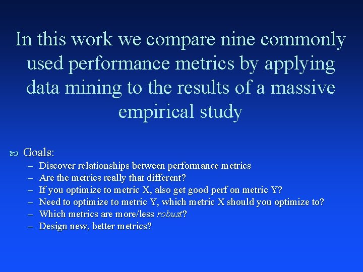
In this work we compare nine commonly used performance metrics by applying data mining to the results of a massive empirical study Goals: – – – Discover relationships between performance metrics Are the metrics really that different? If you optimize to metric X, also get good perf on metric Y? Need to optimize to metric Y, which metric X should you optimize to? Which metrics are more/less robust? Design new, better metrics?

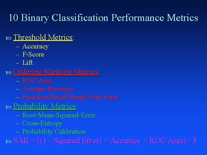
10 Binary Classification Performance Metrics Threshold Metrics: – Accuracy – F-Score – Lift Ordering/Ranking Metrics: – ROC Area – Average Precision – Precision/Recall Break-Even Point Probability Metrics: – Root-Mean-Squared-Error – Cross-Entropy – Probability Calibration SAR = ((1 - Squared Error) + Accuracy + ROC Area) / 3

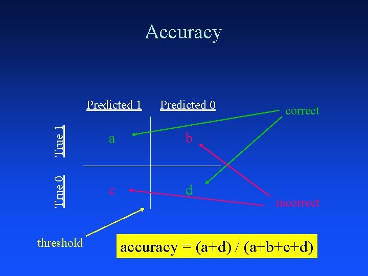
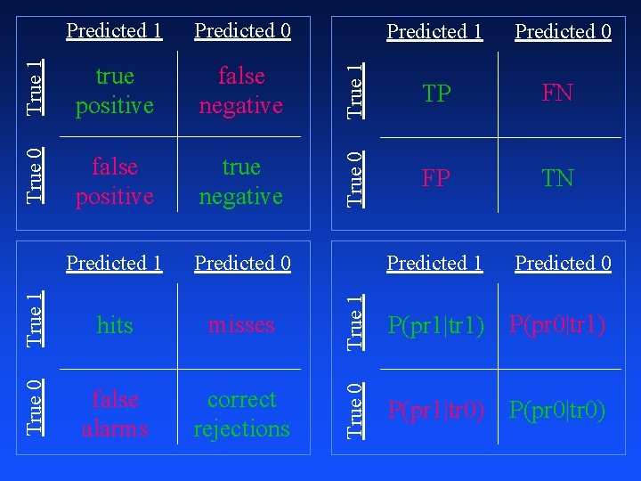
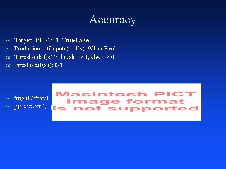
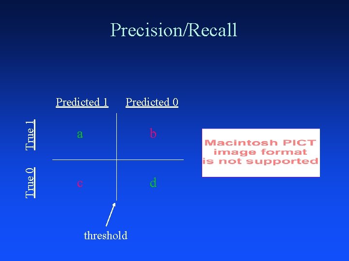
Predicted 1 Predicted 0 True 1 a b True 0 Accuracy c d threshold correct incorrect accuracy = (a+d) / (a+b+c+d)

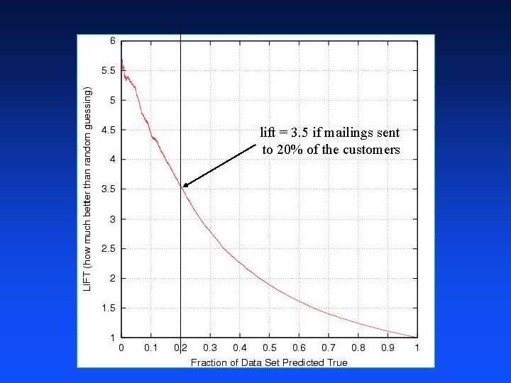
Lift not interested in accuracy on entire dataset want accurate predictions for 5%, 10%, or 20% of dataset don’t care about remaining 95%, 90%, 80%, resp. typical application: marketing how much better than random prediction on the fraction of the dataset predicted true (f(x) > threshold)

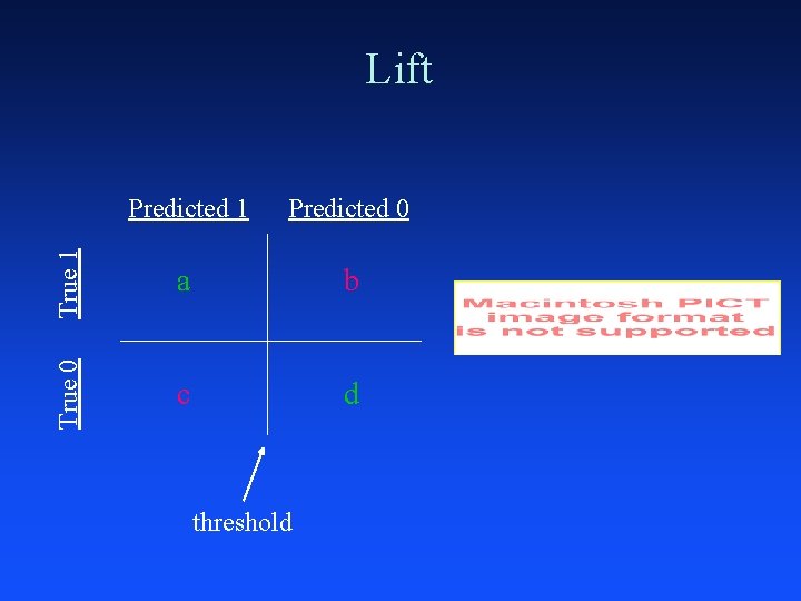
Predicted 1 Predicted 0 True 1 a b True 0 Lift c d threshold

lift = 3. 5 if mailings sent to 20% of the customers

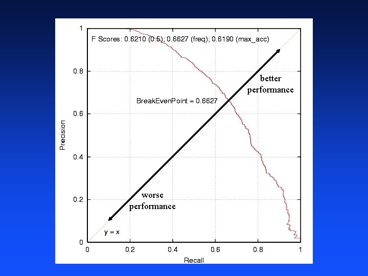
Precision/Recall, F, Break-Even Pt harmonic average of precision and recall

better performance worse performance

True 0 false positive true negative Predicted 1 Predicted 0 True 1 hits misses True 0 false alarms correct rejections True 1 false negative Predicted 0 TP FN True 0 True 1 true positive Predicted 1 FP TN Predicted 1 Predicted 0 True 1 Predicted 0 P(pr 1|tr 1) P(pr 0|tr 1) True 0 Predicted 1 P(pr 1|tr 0) P(pr 0|tr 0)

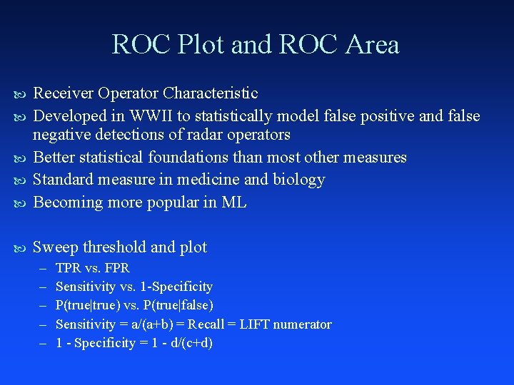
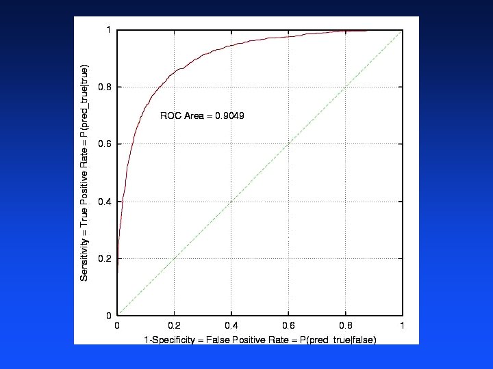
ROC Plot and ROC Area Receiver Operator Characteristic Developed in WWII to statistically model false positive and false negative detections of radar operators Better statistical foundations than most other measures Standard measure in medicine and biology Becoming more popular in ML Sweep threshold and plot – – – TPR vs. FPR Sensitivity vs. 1 -Specificity P(true|true) vs. P(true|false) Sensitivity = a/(a+b) = Recall = LIFT numerator 1 - Specificity = 1 - d/(c+d)

diagonal line is random prediction

Calibration Good If calibration: 1000 x’s have pred(x) = 0. 2, ~200 should be positive

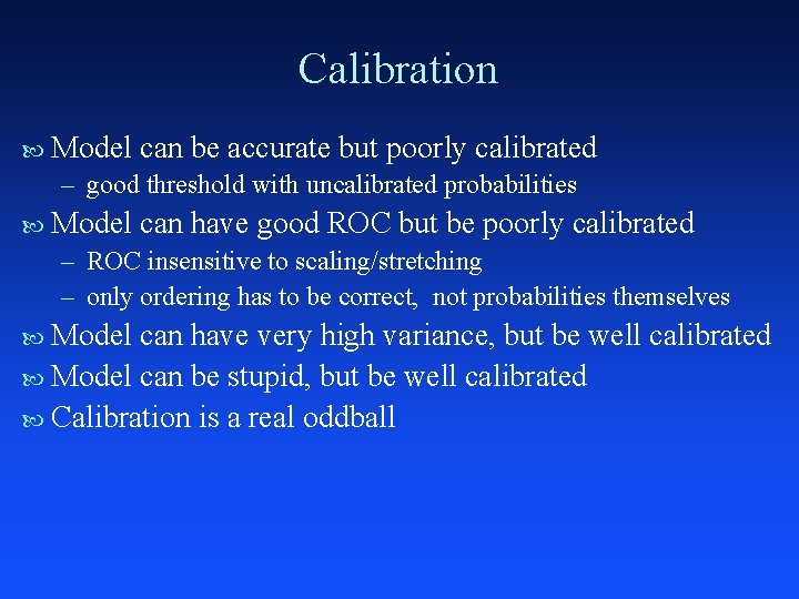
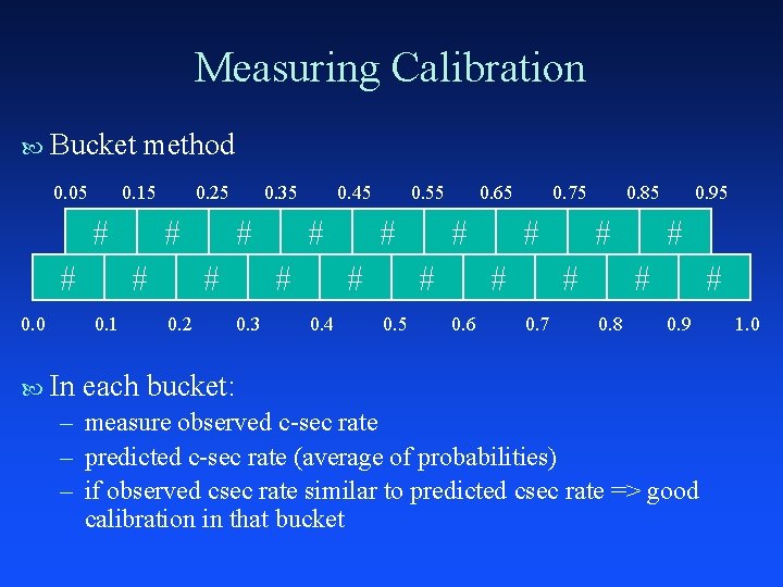
Calibration Model can be accurate but poorly calibrated – good threshold with uncalibrated probabilities Model can have good ROC but be poorly calibrated – ROC insensitive to scaling/stretching – only ordering has to be correct, not probabilities themselves Model can have very high variance, but be well calibrated Model can be stupid, but be well calibrated Calibration is a real oddball

Measuring Calibration Bucket 0. 05 method 0. 15 # # 0. 0 # # 0. 1 In 0. 25 0. 35 # # 0. 2 0. 45 # # 0. 3 0. 55 # # 0. 4 0. 65 # # 0. 5 0. 75 # # 0. 6 0. 85 # # 0. 7 0. 95 # # 0. 8 # 0. 9 each bucket: – measure observed c-sec rate – predicted c-sec rate (average of probabilities) – if observed csec rate similar to predicted csec rate => good calibration in that bucket 1. 0

Calibration Plot

Experiments

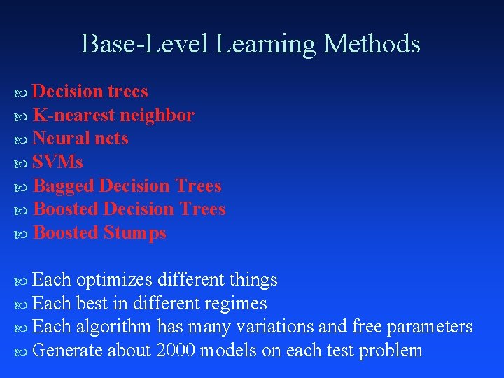
Base-Level Learning Methods Decision trees K-nearest neighbor Neural nets SVMs Bagged Decision Trees Boosted Stumps Each optimizes different things Each best in different regimes Each algorithm has many variations and free parameters Generate about 2000 models on each test problem

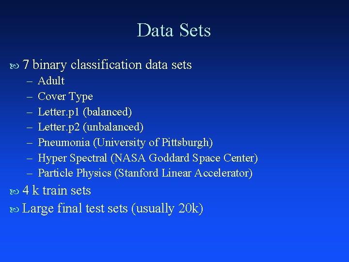
Data Sets 7 binary classification data sets – – – – 4 Adult Cover Type Letter. p 1 (balanced) Letter. p 2 (unbalanced) Pneumonia (University of Pittsburgh) Hyper Spectral (NASA Goddard Space Center) Particle Physics (Stanford Linear Accelerator) k train sets Large final test sets (usually 20 k)

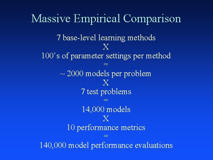
Massive Empirical Comparison 7 base-level learning methods X 100’s of parameter settings per method = ~ 2000 models per problem X 7 test problems = 14, 000 models X 10 performance metrics = 140, 000 model performance evaluations

COVTYPE: Calibration vs. Accuracy

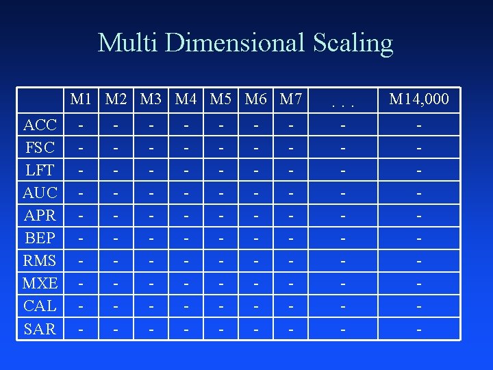
Multi Dimensional Scaling M 1 M 2 M 3 M 4 M 5 M 6 M 7 ACC FSC LFT AUC APR BEP RMS MXE CAL SAR - - - - . . . M 14, 000 - -

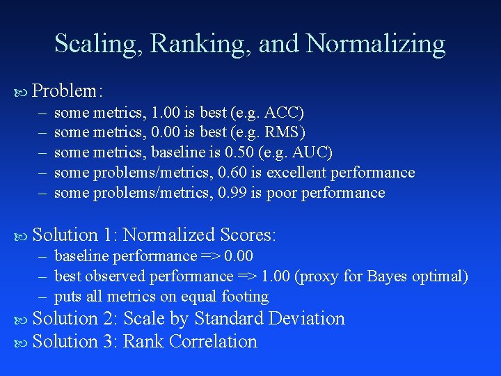
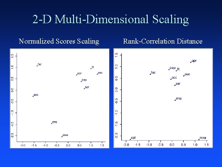
Scaling, Ranking, and Normalizing Problem: – – – some metrics, 1. 00 is best (e. g. ACC) some metrics, 0. 00 is best (e. g. RMS) some metrics, baseline is 0. 50 (e. g. AUC) some problems/metrics, 0. 60 is excellent performance some problems/metrics, 0. 99 is poor performance Solution 1: Normalized Scores: – baseline performance => 0. 00 – best observed performance => 1. 00 (proxy for Bayes optimal) – puts all metrics on equal footing Solution 2: Scale by Standard Deviation Solution 3: Rank Correlation

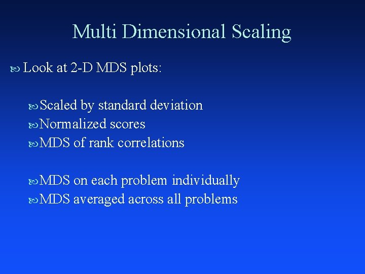
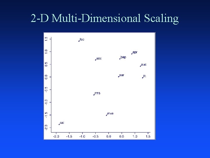
Multi Dimensional Scaling Find low-dimension embedding of 10 x 14, 000 data The 10 metrics span a 2 -5 dimension subspace

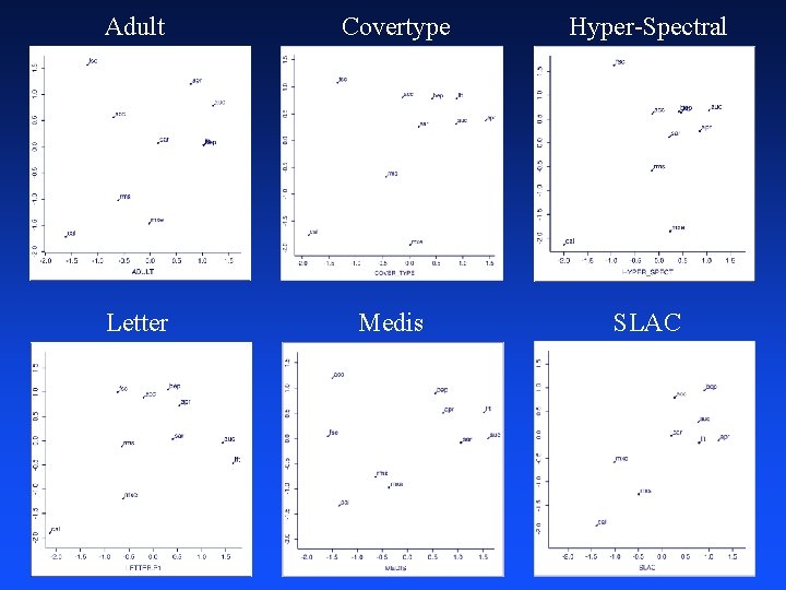
Multi Dimensional Scaling Look at 2 -D MDS plots: Scaled by standard deviation Normalized scores MDS of rank correlations MDS on each problem individually MDS averaged across all problems

2 -D Multi-Dimensional Scaling

2 -D Multi-Dimensional Scaling Normalized Scores Scaling Rank-Correlation Distance

Adult Covertype Hyper-Spectral Letter Medis SLAC

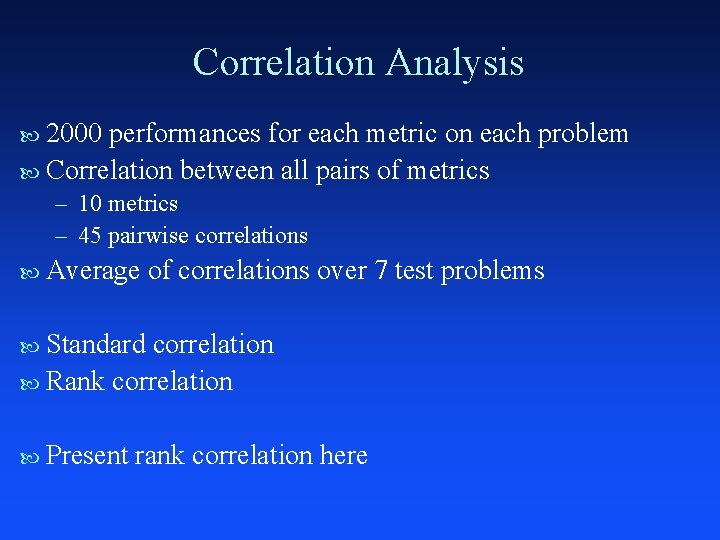
Correlation Analysis 2000 performances for each metric on each problem Correlation between all pairs of metrics – 10 metrics – 45 pairwise correlations Average of correlations over 7 test problems Standard correlation Rank correlation Present rank correlation here

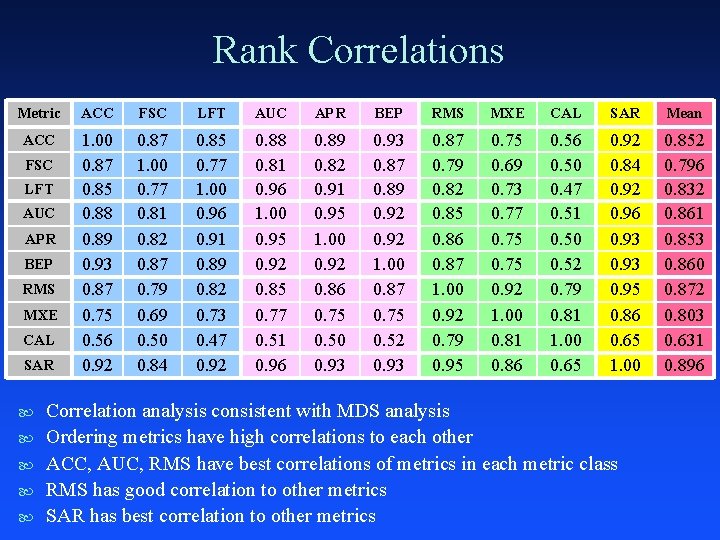
Rank Correlations Metric ACC FSC LFT AUC APR BEP RMS MXE CAL SAR Mean ACC 1. 00 0. 87 0. 85 0. 88 0. 89 0. 93 0. 87 0. 75 0. 56 0. 92 0. 87 1. 00 0. 77 0. 81 0. 82 0. 87 0. 79 0. 69 0. 50 0. 84 0. 85 0. 77 1. 00 0. 96 0. 91 0. 89 0. 82 0. 73 0. 47 0. 92 0. 88 0. 81 0. 96 1. 00 0. 95 0. 92 0. 85 0. 77 0. 51 0. 96 0. 89 0. 82 0. 91 0. 95 1. 00 0. 92 0. 86 0. 75 0. 50 0. 93 0. 87 0. 89 0. 92 1. 00 0. 87 0. 75 0. 52 0. 93 0. 87 0. 79 0. 82 0. 85 0. 86 0. 87 1. 00 0. 92 0. 79 0. 95 0. 75 0. 69 0. 73 0. 77 0. 75 0. 92 1. 00 0. 81 0. 86 0. 50 0. 47 0. 51 0. 50 0. 52 0. 79 0. 81 1. 00 0. 65 0. 92 0. 84 0. 92 0. 96 0. 93 0. 95 0. 86 0. 65 1. 00 0. 852 0. 796 0. 832 0. 861 0. 853 0. 860 0. 872 0. 803 0. 631 0. 896 FSC LFT AUC APR BEP RMS MXE CAL SAR Correlation analysis consistent with MDS analysis Ordering metrics have high correlations to each other ACC, AUC, RMS have best correlations of metrics in each metric class RMS has good correlation to other metrics SAR has best correlation to other metrics

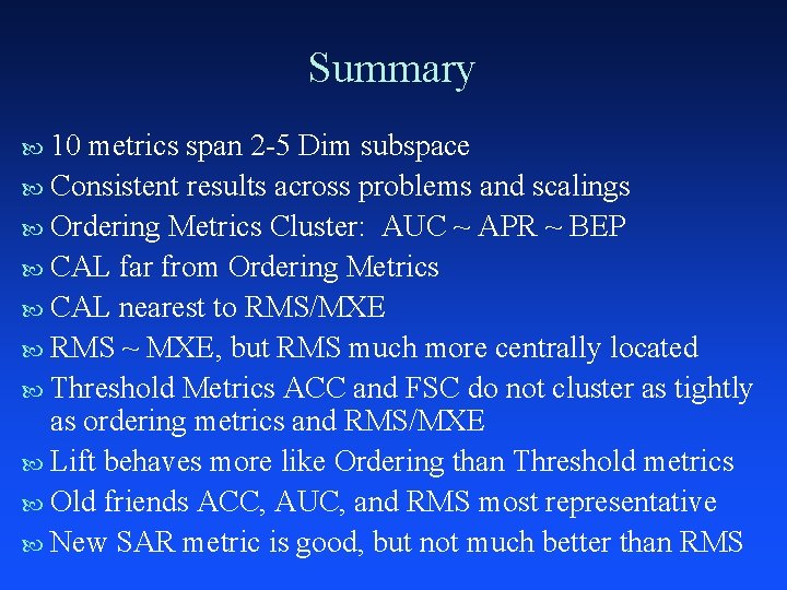
Summary 10 metrics span 2 -5 Dim subspace Consistent results across problems and scalings Ordering Metrics Cluster: AUC ~ APR ~ BEP CAL far from Ordering Metrics CAL nearest to RMS/MXE RMS ~ MXE, but RMS much more centrally located Threshold Metrics ACC and FSC do not cluster as tightly as ordering metrics and RMS/MXE Lift behaves more like Ordering than Threshold metrics Old friends ACC, AUC, and RMS most representative New SAR metric is good, but not much better than RMS

New Resources Want to borrow 14, 000 models? – margin analysis – comparison to new algorithm X – … PERF code: software that calculates ~2 dozen performance metrics: – – – Accuracy (at different thresholds) ROC Area and ROC plots Precision and Recall plots Break-even-point, F-score, Average Precision Squared Error Cross-Entropy Lift … Currently, most metrics are for boolean classification problems We are willing to add new metrics and new capabilities Available at: http: //www. cs. cornell. edu/~caruana

Future Work

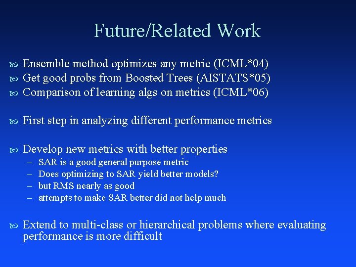
Future/Related Work Ensemble method optimizes any metric (ICML*04) Get good probs from Boosted Trees (AISTATS*05) Comparison of learning algs on metrics (ICML*06) First step in analyzing different performance metrics Develop new metrics with better properties – – SAR is a good general purpose metric Does optimizing to SAR yield better models? but RMS nearly as good attempts to make SAR better did not help much Extend to multi-class or hierarchical problems where evaluating performance is more difficult

Thank You.

Spooky Stuff in Metric Space

Which learning methods perform best on each metric?

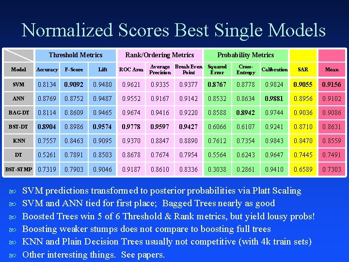
Normalized Scores Best Single Models Threshold Metrics Rank/Ordering Metrics Probability Metrics Average Break Even Precision Point Squared Error Cross. Entropy Calibration SAR Mean 0. 9621 0. 9335 0. 9377 0. 8767 0. 8778 0. 9824 0. 9055 0. 9156 0. 9487 0. 9552 0. 9167 0. 9142 0. 8532 0. 8634 0. 9881 0. 8956 0. 9102 0. 8609 0. 9465 0. 9674 0. 9416 0. 9220 0. 8588 0. 8942 0. 9744 0. 9036 0. 9086 0. 8904 0. 8986 0. 9574 0. 9778 0. 9597 0. 9427 0. 6066 0. 6107 0. 9241 0. 8710 0. 8631 KNN 0. 7557 0. 8463 0. 9095 0. 9370 0. 8847 0. 8890 0. 7612 0. 7354 0. 9843 0. 8470 0. 8559 DT 0. 5261 0. 7891 0. 8503 0. 8678 0. 7674 0. 7954 0. 5564 0. 6243 0. 9647 0. 7445 0. 7491 BST-STMP 0. 7319 0. 7903 0. 9046 0. 9187 0. 8610 0. 8336 0. 3038 0. 2861 0. 9410 0. 6589 0. 7303 Model Accuracy F-Score Lift ROC Area SVM 0. 8134 0. 9092 0. 9480 ANN 0. 8769 0. 8752 BAG-DT 0. 8114 BST-DT SVM predictions transformed to posterior probabilities via Platt Scaling SVM and ANN tied for first place; Bagged Trees nearly as good Boosted Trees win 5 of 6 Threshold & Rank metrics, but yield lousy probs! Boosting weaker stumps does not compare to boosting full trees KNN and Plain Decision Trees usually not competitive (with 4 k train sets) Other interesting things. See papers.

Platt Scaling SVM predictions: [-inf, +inf] Probability metrics require [0, 1] Platt scaling transforms SVM preds by fitting a sigmoid This gives SVM good probability performance

Outline Motivation: The One True Model Ten Performance Metrics Experiments Multidimensional Scaling (MDS) Analysis Correlation Analysis Learning Algorithm vs. Metric Summary

Base-Level Learners Each optimizes different things: – – ANN: minimize squared error or cross-entropy (good for probs) SVM, Boosting: optimize margin (good for accuracy, poor for probs) DT: optimize info gain KNN: ? Each best in different regimes: – SVM: high dimensional data – DT, KNN: large data sets – ANN: non-linear prediction from many correlated features Each algorithm has many variations and free parameters: – – SVM: margin parameter, kernel parameters (gamma, …) ANN: # hidden units, # hidden layers, learning rate, early stopping point DT: splitting criterion, pruning options, smoothing options, … KNN: K, distance metric, distance weighted averaging, … Generate about 2000 models on each test problem

Motivation Holy – – Grail of Supervised Learning: One True Model (a. k. a. Bayes Optimal Model) Predicts correct conditional probability for each case Yields optimal performance on all reasonable metrics Hard to learn given finite data Ç train sets rarely have conditional probs, usually just 0/1 targets – Isn’t always necessary Many – – Different Performance Metrics: ACC, AUC, CXE, RMS, PRE/REC … Each represents different tradeoffs Usually important to optimize to appropriate metric Not all metric created equal

Motivation In an ideal world: – Learn model that predicts correct conditional probabilities – Yield optimal performance on any reasonable metric In real world: – – – Finite data 0/1 targets instead of conditional probabilities Hard to learn this ideal model Don’t have good metrics for recognizing ideal model Ideal model isn’t always necessary In practice: – Do learning using many different metrics: ACC, AUC, CXE, RMS, … – Each metric represents different tradeoffs – Because of this, usually important to optimize to appropriate metric

Accuracy Target: 0/1, -1/+1, True/False, … Prediction = f(inputs) = f(x): 0/1 or Real Threshold: f(x) > thresh => 1, else => 0 threshold(f(x)): 0/1 #right / #total p(“correct”): p(threshold(f(x)) = target)

Precision and Recall Typically used in document retrieval Precision: – how many of the returned documents are correct – precision(threshold) Recall: – how many of the positives does the model return – recall(threshold) Precision/Recall Curve: sweep thresholds

Predicted 1 Predicted 0 True 1 a b True 0 Precision/Recall c d threshold