SPM short course May 2003 Linear Models and

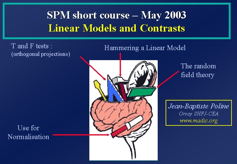
SPM short course – May 2003 Linear Models and Contrasts T and F tests : (orthogonal projections) Hammering a Linear Model The random field theory Jean-Baptiste Poline Orsay SHFJ-CEA Use for Normalisation www. madic. org

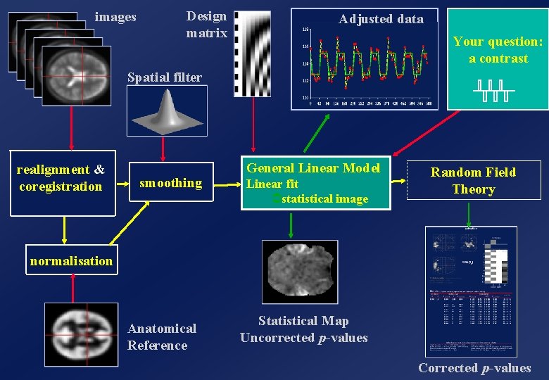
images Design matrix Adjusted data Your question: a contrast Spatial filter realignment & coregistration smoothing General Linear Model Linear fit Üstatistical image Random Field Theory normalisation Anatomical Reference Statistical Map Uncorrected p-values Corrected p-values

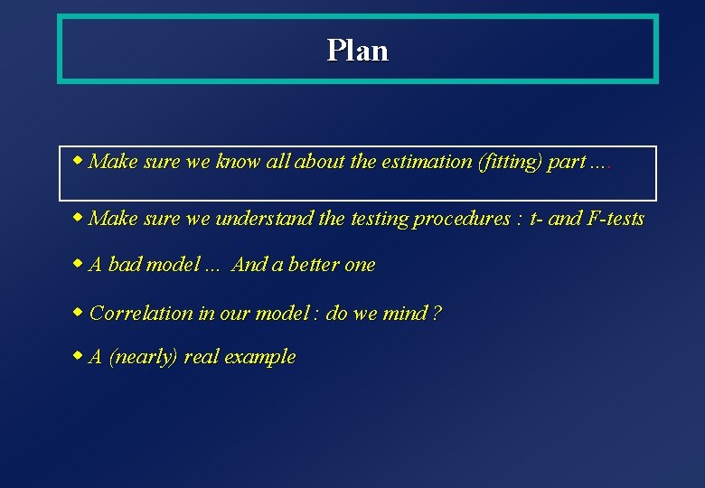
Plan w Make sure we know all about the estimation (fitting) part. . w Make sure we understand the testing procedures : t- and F-tests w A bad model. . . And a better one w Correlation in our model : do we mind ? w A (nearly) real example

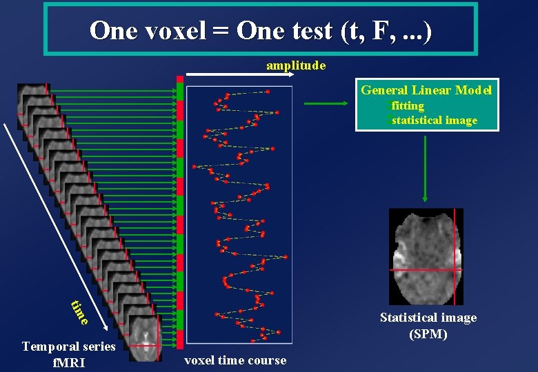
One voxel = One test (t, F, . . . ) amplitude General Linear Model Üfitting Üstatistical image tim e Statistical image (SPM) Temporal series f. MRI voxel time course

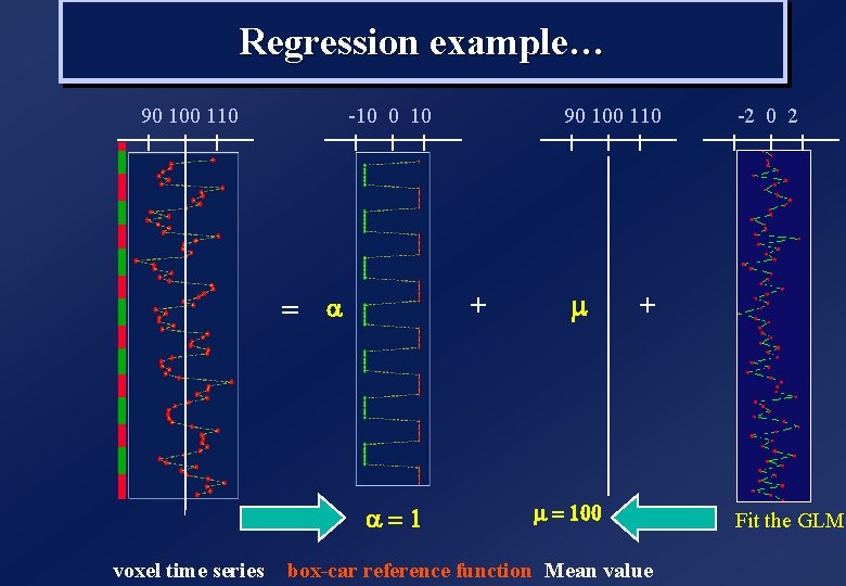
Regression example… 90 100 110 -10 0 10 + = a a=1 voxel time series 90 100 110 m -2 0 2 + m = 100 box-car reference function Mean value Fit the GLM

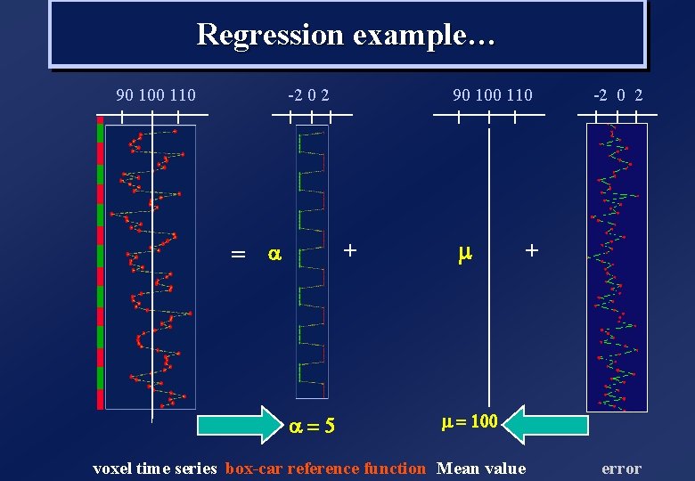
Regression example… 90 100 110 -2 0 2 + = a a=5 m -2 0 2 + m = 100 voxel time series box-car reference function Mean value error

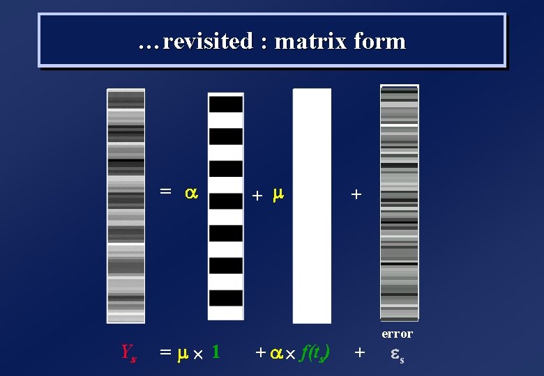
…revisited : matrix form = a Ys = m´ 1 + m + a ´ f(ts) + error + es

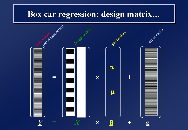
Y = = X ´ ´ b r to ec rv ro er s x er ie ri at er m et m ra pa n de sig (v vec ox to el r tim es ta da s) Box car regression: design matrix… a + m + e

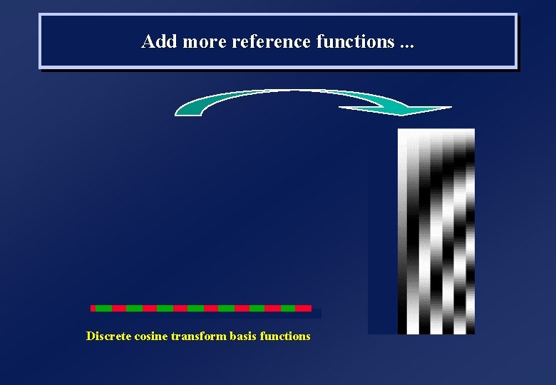
Add more reference functions. . . Discrete cosine transform basis functions

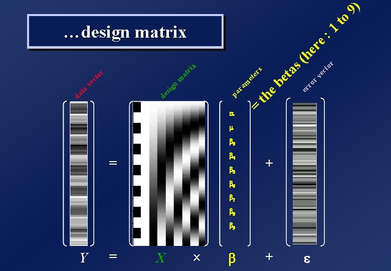
Y = X a = b 4 b 5 ´ b = s + r to ec rv ro er he re s( eb et a th ri x er et at m m ra pa n or ct ve de sig ta da : 1 to …design matrix m b 3 + b 6 b 7 b 8 b 9 e 9)

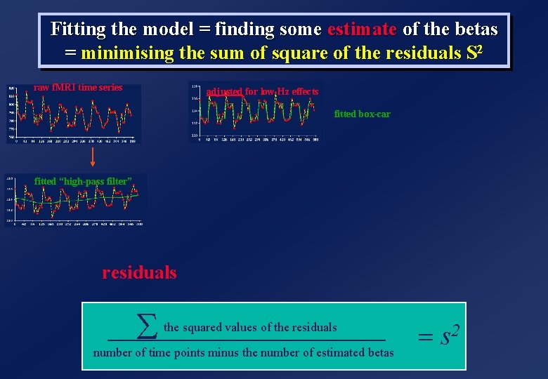
Fitting the model = finding some estimate of the betas = minimising the sum of square of the residuals S 2 raw f. MRI time series adjusted for low Hz effects fitted box-car fitted “high-pass filter” residuals S the squared values of the residuals number of time points minus the number of estimated betas = s 2

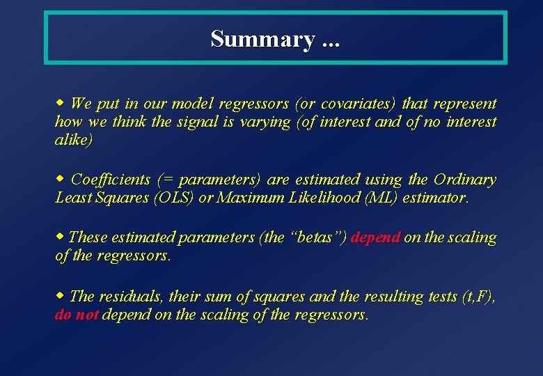
Summary. . . w We put in our model regressors (or covariates) that represent how we think the signal is varying (of interest and of no interest alike) w Coefficients (= parameters) are estimated using the Ordinary Least Squares (OLS) or Maximum Likelihood (ML) estimator. w These estimated parameters (the “betas”) depend on the scaling of the regressors. w The residuals, their sum of squares and the resulting tests (t, F), do not depend on the scaling of the regressors.

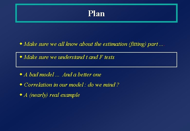
Plan w Make sure we all know about the estimation (fitting) part. . w Make sure we understand t and F tests w A bad model. . . And a better one w Correlation in our model : do we mind ? w A (nearly) real example

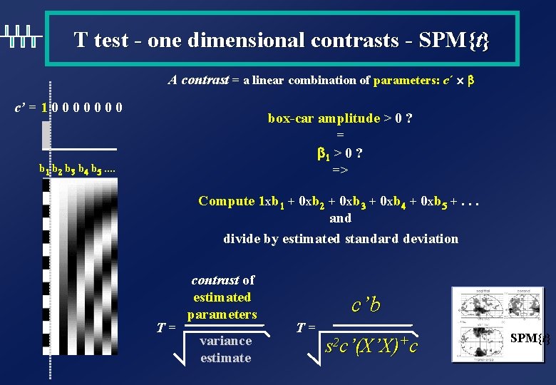
T test - one dimensional contrasts - SPM{t} A contrast = a linear combination of parameters: c´ ´ b c’ = 1 0 0 0 0 box-car amplitude > 0 ? = b 1 > 0 ? => b 1 b 2 b 3 b 4 b 5. . Compute 1 xb 1 + 0 xb 2 + 0 xb 3 + 0 xb 4 + 0 xb 5 +. . . and divide by estimated standard deviation T= contrast of estimated parameters variance estimate c’b T= s 2 c’(X’X)+c SPM{t}

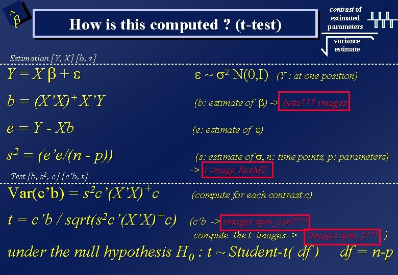
^ b How is this computed ? (t-test) contrast of estimated parameters variance estimate Estimation [Y, X] [b, s] Y=Xb+e e ~ s 2 N(0, I) b = (X’X)+ X’Y (b: estimate of b) -> beta? ? ? images e = Y - Xb (e: estimate of e) s 2 = (e’e/(n - p)) (s: estimate of s, n: time points, p: parameters) -> 1 image Res. MS Test [b, s 2, c] [c’b, t] Var(c’b) = s 2 c’(X’X)+c t = c’b / sqrt(s 2 c’(X’X)+c) (Y : at one position) (compute for each contrast c) (c’b -> images spm_con? ? ? compute the t images -> images spm_t? ? ? ) under the null hypothesis H 0 : t ~ Student-t( df ) df = n-p

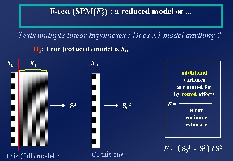
F-test (SPM{F}) : a reduced model or. . . Tests multiple linear hypotheses : Does X 1 model anything ? H 0: True (reduced) model is X 0 X 0 X 1 additional variance accounted for by tested effects S 2 This (full) model ? S 02 Or this one? F= error variance estimate F ~ ( S 02 - S 2 ) / S 2

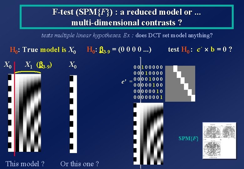
F-test (SPM{F}) : a reduced model or. . . multi-dimensional contrasts ? tests multiple linear hypotheses. Ex : does DCT set model anything? H 0: True model is X 0 X 1 (b 3 -9) H 0: b 3 -9 = (0 0 0 0. . . ) X 0 c’ test H 0 : c´ ´ b = 0 ? 00100000 00010000 =0 0 1 0 00000100 00000010 00000001 SPM{F} This model ? Or this one ?

How is this computed ? (F-test) Estimation [Y, X] [b, s] Y=Xb+e Y = X 0 b 0 + e 0 Estimation [Y, X 0] [b 0, s 0] b 0 = (X 0’X 0)+ X 0’Y e 0 = Y - X 0 b 0 s 20 = (e 0’e 0/(n - p 0)) additional variance accounted for by tested effects Error variance estimate e ~ N(0, s 2 I) e 0 ~ N(0, s 02 I) X 0 : X Reduced (eà: estimate of eà) (sà: estimate of sà, n: time, pà: parameters) Test [b, s, c] [ess, F] F = (e 0’e 0 - e’e)/(p - p 0) / s 2 -> image (e 0’e 0 - e’e)/(p - p 0) : spm_ess? ? ? -> image of F : spm_F? ? ? under the null hypothesis : F ~ F(df 1, df 2) p - p 0 n-p

Plan w Make sure we all know about the estimation (fitting) part. . w Make sure we understand t and F tests w A bad model. . . And a better one w Correlation in our model : do we mind ? w A (nearly) real example

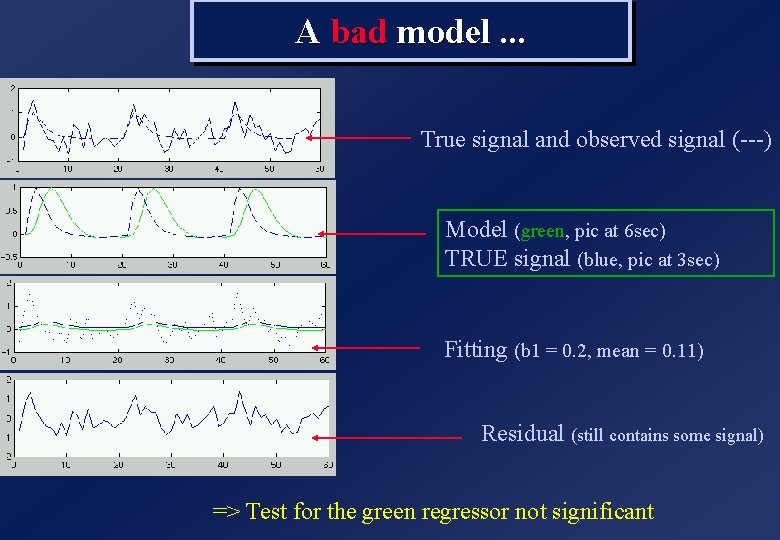
A bad model. . . True signal and observed signal (---) Model (green, pic at 6 sec) TRUE signal (blue, pic at 3 sec) Fitting (b 1 = 0. 2, mean = 0. 11) Residual (still contains some signal) => Test for the green regressor not significant

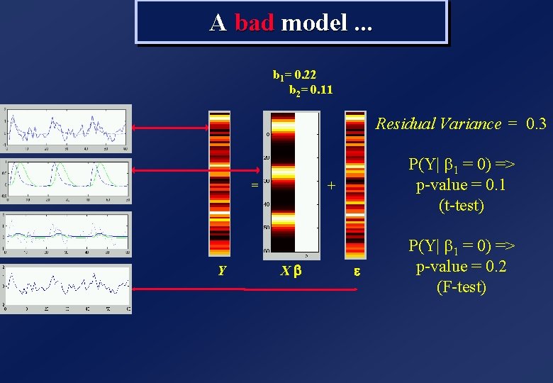
A bad model. . . b 1= 0. 22 b 2= 0. 11 Residual Variance = 0. 3 = Y P(Y| b 1 = 0) => p-value = 0. 1 (t-test) + Xb e P(Y| b 1 = 0) => p-value = 0. 2 (F-test)

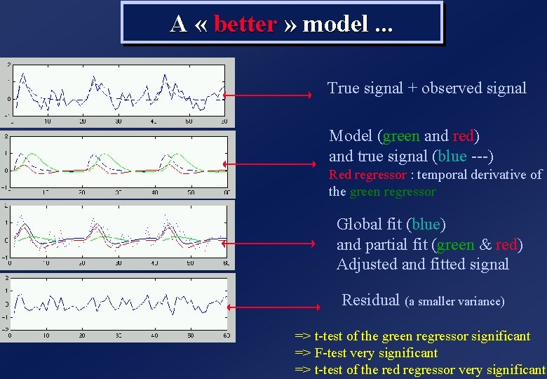
A « better » model. . . True signal + observed signal Model (green and red) and true signal (blue ---) Red regressor : temporal derivative of the green regressor Global fit (blue) and partial fit (green & red) Adjusted and fitted signal Residual (a smaller variance) => t-test of the green regressor significant => F-test very significant => t-test of the red regressor very significant

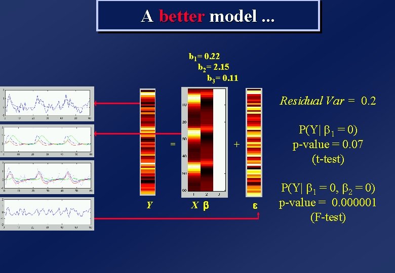
A better model. . . b 1= 0. 22 b 2= 2. 15 b 3= 0. 11 Residual Var = 0. 2 = Y P(Y| b 1 = 0) p-value = 0. 07 (t-test) + X b e P(Y| b 1 = 0, b 2 = 0) p-value = 0. 000001 (F-test)

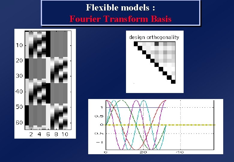
Flexible models : Fourier Transform Basis

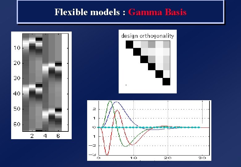
Flexible models : Gamma Basis

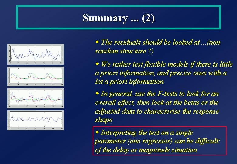
Summary. . . (2) w The residuals should be looked at. . . (non random structure ? ) w We rather test flexible models if there is little a priori information, and precise ones with a lot a priori information w In general, use the F-tests to look for an overall effect, then look at the betas or the adjusted data to characterise the response shape w Interpreting the test on a single parameter (one regressor) can be difficult: cf the delay or magnitude situation

Plan w Make sure we all know about the estimation (fitting) part. . w Make sure we understand t and F tests w A bad model. . . And a better one w Correlation in our model : do we mind ? w A (nearly) real example ?

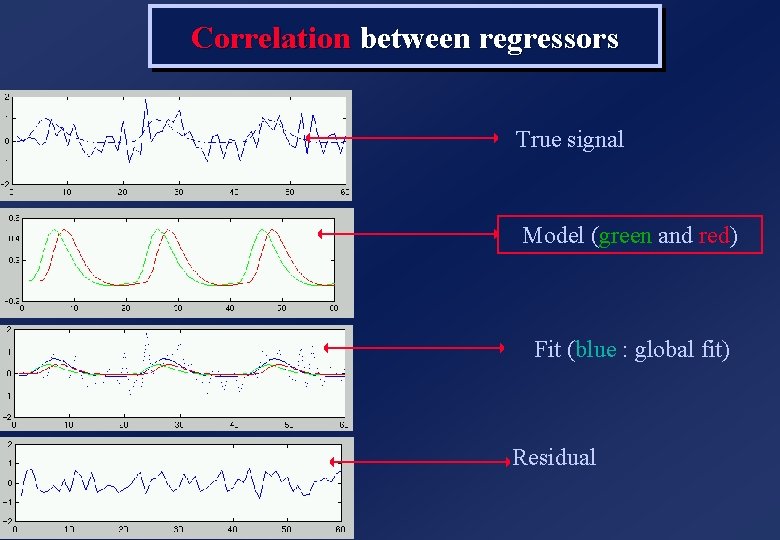
Correlation between regressors True signal Model (green and red) Fit (blue : global fit) Residual

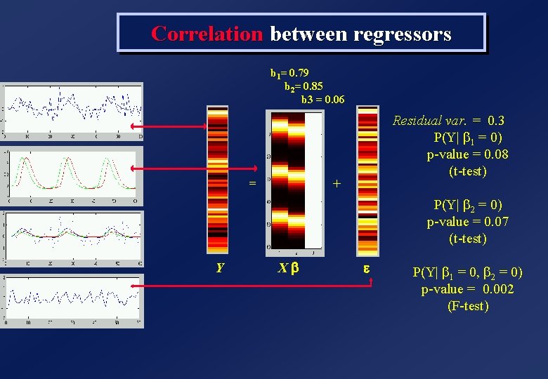
Correlation between regressors b 1= 0. 79 b 2= 0. 85 b 3 = 0. 06 = Residual var. = 0. 3 P(Y| b 1 = 0) p-value = 0. 08 (t-test) + P(Y| b 2 = 0) p-value = 0. 07 (t-test) Y Xb e P(Y| b 1 = 0, b 2 = 0) p-value = 0. 002 (F-test)

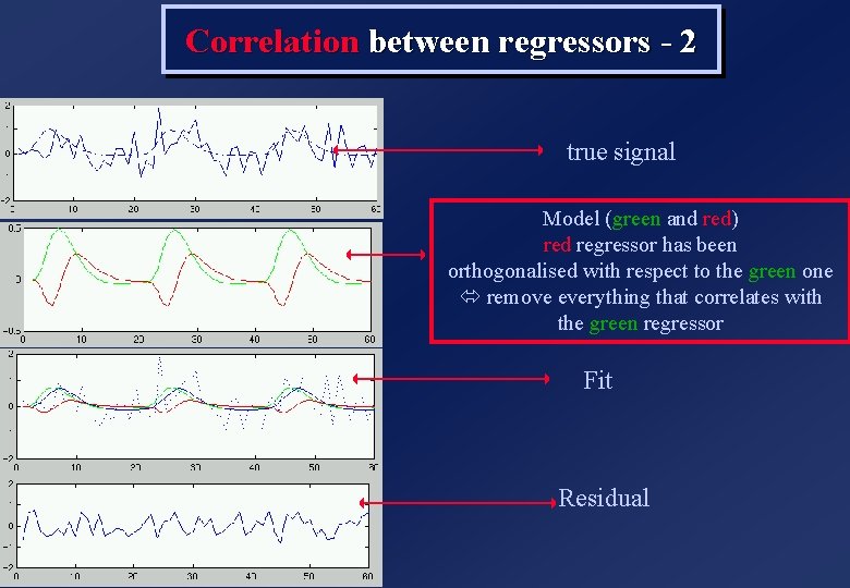
Correlation between regressors - 2 true signal Model (green and red) red regressor has been orthogonalised with respect to the green one remove everything that correlates with the green regressor Fit Residual

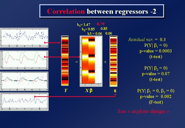
Correlation between regressors -2 0. 79 b 1= 1. 47 0. 85 b 2= 0. 85 b 3 = 0. 06 Residual var. = 0. 3 P(Y| b 1 = 0) p-value = 0. 0003 (t-test) = + P(Y| b 2 = 0) p-value = 0. 07 (t-test) Y Xb e P(Y| b 1 = 0, b 2 = 0) p-value = 0. 002 (F-test) See « explore design »

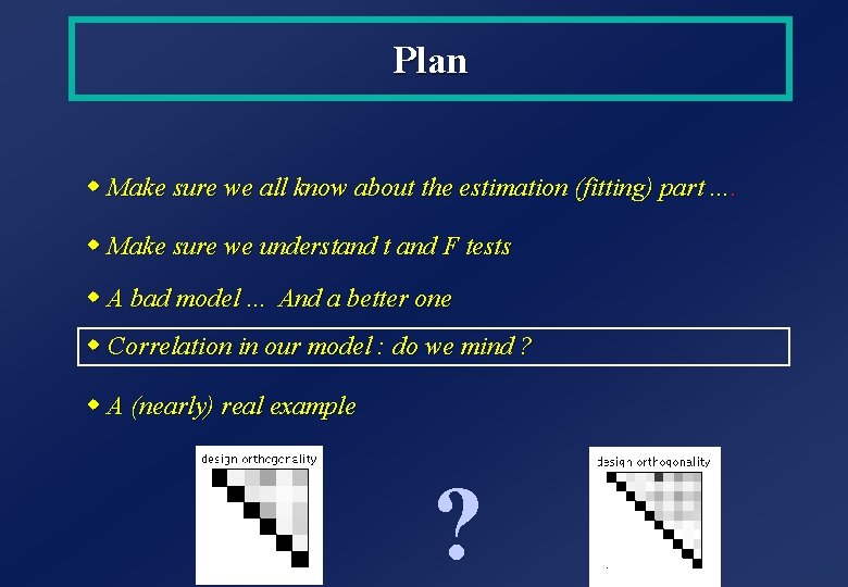
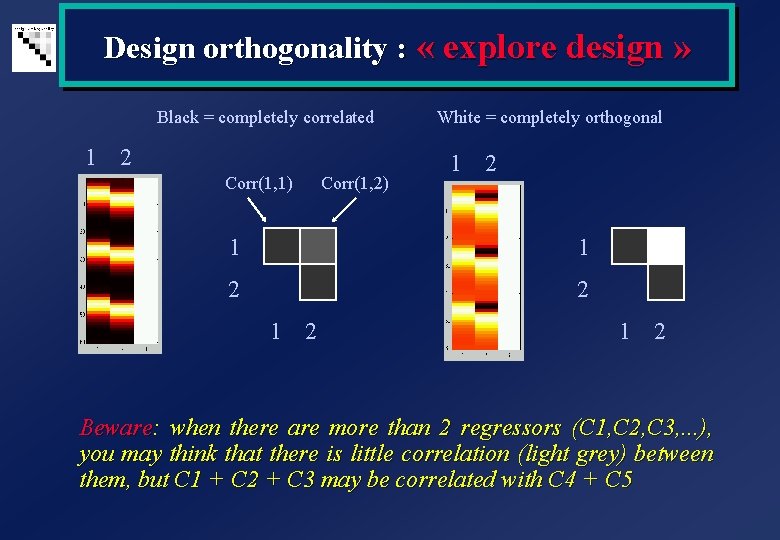
Design orthogonality : « explore design » Black = completely correlated 1 2 Corr(1, 1) Corr(1, 2) White = completely orthogonal 1 2 1 1 2 2 1 2 Beware: when there are more than 2 regressors (C 1, C 2, C 3, . . . ), you may think that there is little correlation (light grey) between them, but C 1 + C 2 + C 3 may be correlated with C 4 + C 5

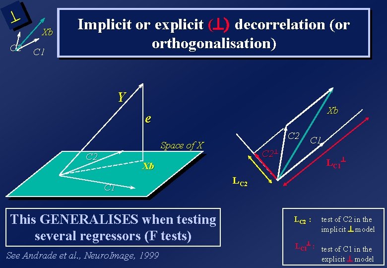
^ C 2 Xb C 1 Implicit or explicit (^) decorrelation (or orthogonalisation) Y Xb e C 2 Space of X C 2 C 1 C 2^ LC 1^ Xb C 1 This GENERALISES when testing several regressors (F tests) See Andrade et al. , Neuro. Image, 1999 LC 2 : test of C 2 in the implicit ^ model LC 1^ : test of C 1 in the explicit ^ model

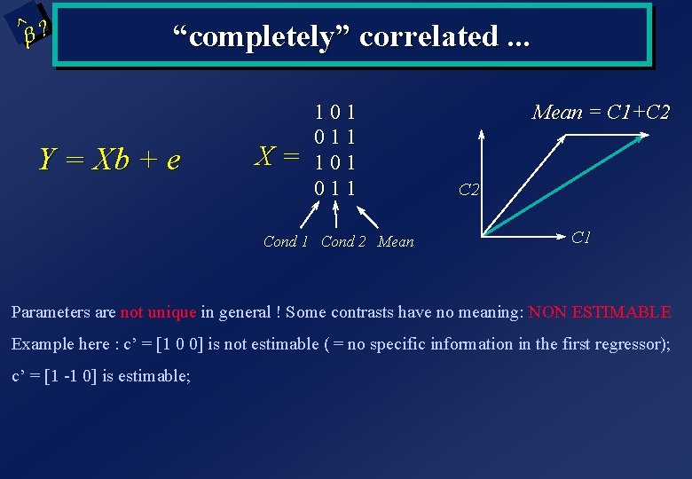
^ ? b “completely” correlated. . . Y = Xb + e X= 101 011 Cond 2 Mean = C 1+C 2 C 1 Parameters are not unique in general ! Some contrasts have no meaning: NON ESTIMABLE Example here : c’ = [1 0 0] is not estimable ( = no specific information in the first regressor); c’ = [1 -1 0] is estimable;

Summary. . . (3) w We implicitly test for an additional effect only, so we may miss the signal if there is some correlation in the model w Orthogonalisation is not generally needed - parameters and test on the changed regressor don’t change w It is always simpler (if possible!) to have orthogonal regressors w In case of correlation, use F-tests to see the overall significance. There is generally no way to decide to which regressor the « common » part should be attributed to w In case of correlation and if you need to orthogonolise a part of the design matrix, there is no need to re-fit a new model: change the contrast

Plan w Make sure we all know about the estimation (fitting) part. . w Make sure we understand t and F tests w A bad model. . . And a better one w Correlation in our model : do we mind ? w A (nearly) real example

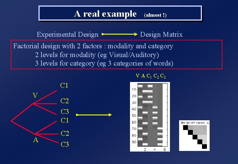
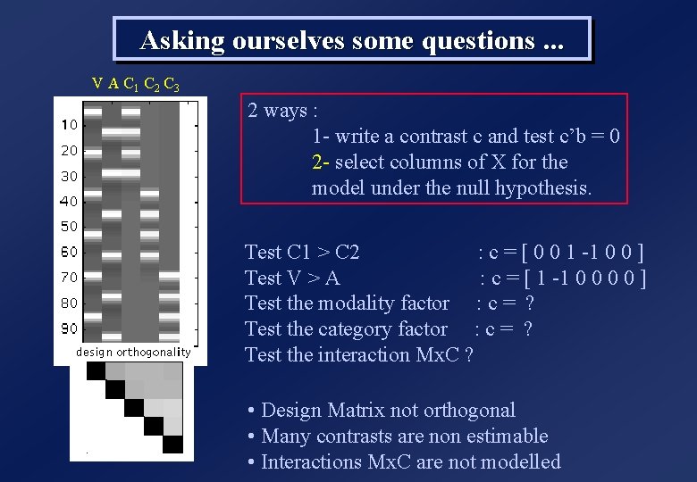
A real example Experimental Design (almost !) Design Matrix Factorial design with 2 factors : modality and category 2 levels for modality (eg Visual/Auditory) 3 levels for category (eg 3 categories of words) V A C 1 C 2 C 3 C 1 V A C 2 C 3 C 1 C 2 C 3

Asking ourselves some questions. . . V A C 1 C 2 C 3 2 ways : 1 - write a contrast c and test c’b = 0 2 - select columns of X for the model under the null hypothesis. Test C 1 > C 2 : c = [ 0 0 1 -1 0 0 ] Test V > A : c = [ 1 -1 0 0 ] Test the modality factor : c = ? Test the category factor : c = ? Test the interaction Mx. C ? • Design Matrix not orthogonal • Many contrasts are non estimable • Interactions Mx. C are not modelled

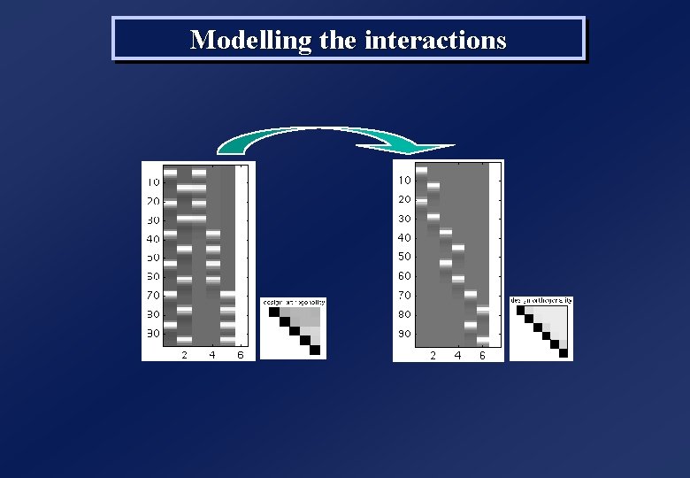
Modelling the interactions

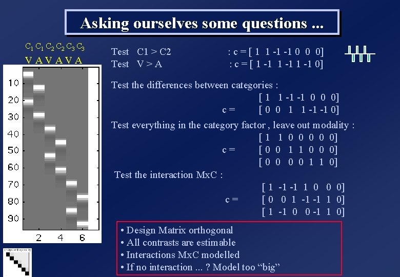
Asking ourselves some questions. . . C 1 C 2 C 3 VAVAVA Test C 1 > C 2 Test V > A : c = [ 1 1 -1 -1 0 0 0] : c = [ 1 -1 0] Test the differences between categories : [ 1 1 -1 -1 0 0 0] c= [ 0 0 1 1 -1 -1 0] Test everything in the category factor , leave out modality : [ 1 1 0 0 0] c= [ 0 0 1 1 0 0 0] [ 0 0 1 1 0] Test the interaction Mx. C : [ 1 -1 -1 1 0 0 0] c= [ 0 0 1 -1 -1 1 0] [ 1 -1 0 0 -1 1 0] • Design Matrix orthogonal • All contrasts are estimable • Interactions Mx. C modelled • If no interaction. . . ? Model too “big”

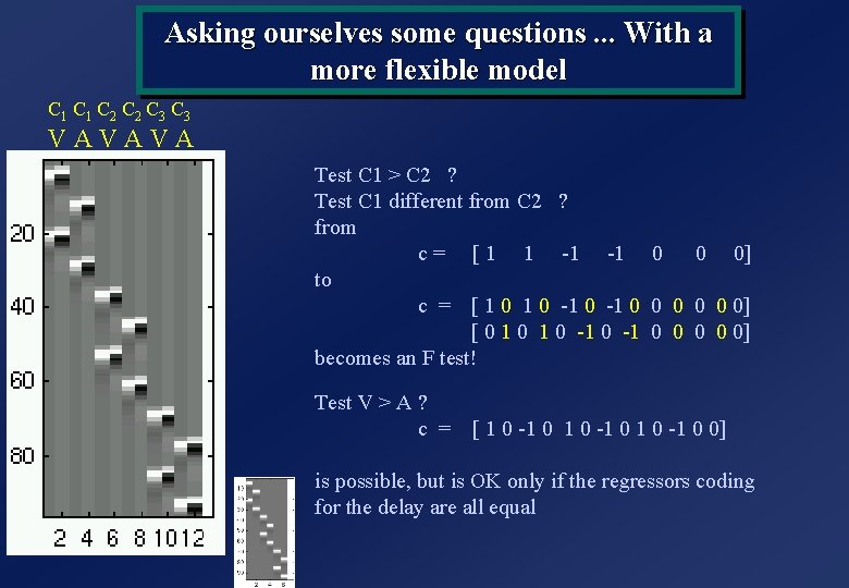
Asking ourselves some questions. . . With a more flexible model C 1 C 2 C 3 VAVAVA Test C 1 > C 2 ? Test C 1 different from C 2 ? from c = [ 1 1 -1 -1 0 0 0] to c = [ 1 0 -1 0 0 0 0] [ 0 1 0 -1 0 0 0] becomes an F test! Test V > A ? c = [ 1 0 -1 0 0] is possible, but is OK only if the regressors coding for the delay are all equal

Conclusion w Check your models w Toolbox of T. Nichols w Multivariate Methods toolbox (F. Kherif, JB Poline et al) w Check the form of the HRF : non parametric estimation www. fil. ion. ucl. ac. uk; www. madic. org; others …