SPM Course Oct 2011 VoxelBased Morphometry Ged Ridgway

SPM Course Oct 2011 Voxel-Based Morphometry Ged Ridgway With thanks to John Ashburner and the FIL Methods Group

Aims of computational neuroanatomy * Many interesting and clinically important questions might relate to the shape or local size of regions of the brain * For example, whether (and where) local patterns of brain morphometry help to: * * * Distinguish schizophrenics from healthy controls Explain the changes seen in development and aging Understand plasticity, e. g. when learning new skills Find structural correlates (scores, traits, genetics, etc. ) Differentiate degenerative disease from healthy aging * Evaluate subjects on drug treatments versus placebo

SPM for group f. MRI Group-wise statistics f. MRI time-series Preprocessing Stat. modelling Results query “Contrast” spm T Image Preprocessing Stat. modelling Results query “Contrast” Image f. MRI time-series

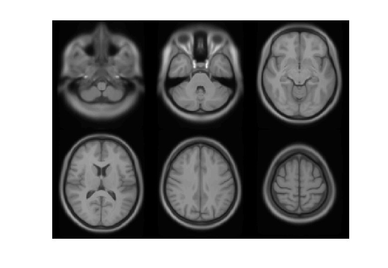
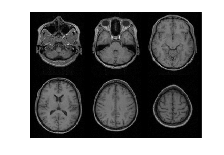
SPM for structural MRI High-res T 1 MRI ? ? Group-wise statistics

Segmentation into principal tissue types * High-resolution MRI reveals fine structural detail in the brain, but not all of it reliable or interesting * Noise, intensity-inhomogeneity, vasculature, … * MR Intensity is usually not quantitatively meaningful (in the same way that e. g. CT is) * f. MRI time-series allow signal changes to be analysed statistically, compared to baseline or global values * Regional volumes of the three main tissue types: gray matter, white matter and CSF, are well-defined and potentially very interesting * Other aspects (and other sequences) can also be of interest

Summary of unified segmentation * Unifies tissue segmentation and spatial normalisation * Principled Bayesian formulation: probabilistic generative model * Gaussian mixture model with deformable tissue prior probability maps (from segmentations in MNI space) * The inverse of the transformation that aligns the TPMs can be used to normalise the original image to standard space * Bias correction is included within the model

Modelling inhomogeneity * MR images are corrupted by spatially smooth intensity variations (worse at high field strength) * A multiplicative bias correction field is modelled as a linear combination of basis functions. Corrupted image Bias Field Corrected image
 * Classification is based on a Mixture")
Gaussian mixture model (GMM or Mo. G) * Classification is based on a Mixture of Gaussians (Mo. G) model fitted to the intensity probability density (histogram) Frequency Image Intensity
")
Tissue intensity distributions (T 1 -w MRI)

Non-Gaussian Intensity Distributions * Multiple Gaussians per tissue class allow non-Gaussian intensity distributions to be modelled. * E. g. accounting for partial volume effects

TPMs – Tissue prior probability maps * Each TPM indicates the prior probability for a particular tissue at each point in MNI space * Fraction of occurrences in previous segmentations * TPMs are warped to match the subject * The inverse transform normalises to MNI space

Voxel-Based Morphometry * In essence VBM is Statistical Parametric Mapping of regional segmented tissue density or volume * The exact interpretation of gray matter density or volume is complicated, and depends on the preprocessing steps used * It is not interpretable as neuronal packing density or other cytoarchitectonic tissue properties * The hope is that changes in these microscopic properties may lead to macro- or mesoscopic VBM-detectable differences

VBM methods overview * Unified segmentation and spatial normalisation * More flexible groupwise normalisation using DARTEL * * [Optional] modulation with Jacobian determinant Optional computation of tissue totals/globals Gaussian smoothing Voxel-wise statistical analysis

VBM in pictures Segment Normalise

VBM in pictures Segment Normalise Modulate Smooth

VBM in pictures Segment Normalise Modulate Smooth Voxel-wise statistics

VBM in pictures beta_0001 con_0001 Res. MS spm. T_0001 Segment Normalise Modulate Smooth Voxel-wise statistics FWE < 0. 05

VBM Subtleties * * * Whether to modulate How much to smooth Interpreting results Adjusting for total GM or Intracranial Volume Limitations of linear correlation Statistical validity
")
Modulation Native 1 intensity = tissue density 1 * Multiplication of the warped (normalised) tissue intensities so that their regional or global volume is preserved * Can detect differences in completely registered areas * Otherwise, we preserve concentrations, and are detecting mesoscopic effects that remain after approximate registration has removed the macroscopic effects Unmodulated 1 1 Modulated * Flexible (not necessarily “perfect”) registration may not leave any such differences 2/3 1/3 2/3
 =")
Modulation tutorial X=x 2 X’ = d. X/dx = 2 x X’(2. 5) = 5 Available from http: //tinyurl. com/Modulation. Tutorial
(r+s) = pr+ps+qr+qs Red area = Square – cyan")
Modulation tutorial Square area = (p+q)(r+s) = pr+ps+qr+qs Red area = Square – cyan – magenta – green = pr+ps+qr+qs – 2 qr – qs – pr = ps – qr

Smoothing * The analysis will be most sensitive to effects that match the shape and size of the kernel * The data will be more Gaussian and closer to a continuous random field for larger kernels * Results will be rough and noise-like if too little smoothing is used * Too much will lead to distributed, indistinct blobs

Smoothing * Between 7 and 14 mm is probably reasonable * (DARTEL’s greater precision allows less smoothing) * The results below show two fairly extreme choices, 5 mm on the left, and 16 mm, right

Interpreting findings Mis-classify Mis-register Folding Thickening Thinning Mis-register Mis-classify

“Globals” for VBM * Shape is really a multivariate concept * Dependencies among volumes in different regions * SPM is mass univariate * Combining voxel-wise information with “global” integrated tissue volume provides a compromise * Using either ANCOVA or proportional scaling (ii) is globally thicker, but locally thinner than (i) – either of these effects may be of interest to us. Fig. from: Voxel-based morphometry of the human brain… Mechelli, Price, Friston and Ashburner. Current Medical Imaging Reviews 1(2), 2005.
 * “Global” integrated tissue volume may be correlated with interesting")
Total Intracranial Volume (TIV/ICV) * “Global” integrated tissue volume may be correlated with interesting regional effects * Correcting for globals in this case may overly reduce sensitivity to local differences * Total intracranial volume integrates GM, WM and CSF, or attempts to measure the skull-volume directly * Not sensitive to global reduction of GM+WM (cancelled out by CSF expansion – skull is fixed!) * Correcting for TIV in VBM statistics may give more powerful and/or more interpretable results * See e. g. Barnes et al. , (2010), Neuro. Image 53(4): 1244 -55

VBM’s statistical validity * Residuals are not normally distributed * Little impact on uncorrected statistics for experiments comparing reasonably sized groups * Probably invalid for experiments that compare single subjects or tiny patient groups with a larger control group * Mitigate with large amounts of smoothing * Or use nonparametric tests that make fewer assumptions, e. g. permutation testing with Sn. PM

VBM’s statistical validity * Correction for multiple comparisons * RFT correction based on peak heights is fine * Correction using cluster extents is problematic * SPM usually assumes that the smoothness of the residuals is spatially stationary * VBM residuals have spatially varying smoothness * Bigger blobs expected in smoother regions * Cluster-based correction accounting for nonstationary smoothness is under development * See also Satoru Hayasaka’s nonstationarity toolbox http: //www. fmri. wfubmc. edu/cms/NS-General * Or use Sn. PM…

VBM’s statistical validity * False discovery rate * Less conservative than FWE * Popular in morphometric work * (almost universal for cortical thickness in Free. Surfer) * Recently questioned… * Topological FDR (for clusters and peaks) * See SPM 8 release notes and Justin’s papers * http: //dx. doi. org/10. 1016/j. neuroimage. 2008. 05. 021 * http: //dx. doi. org/10. 1016/j. neuroimage. 2009. 10. 090

Longitudinal VBM * The simplest method for longitudinal VBM is to use cross -sectional preprocessing, but longitudinal statistical analyses * Standard preprocessing not optimal, but unbiased * Non-longitudinal statistics would be severely biased * (Estimates of standard errors would be too small) * Simplest longitudinal statistical analysis: two-stage summary statistic approach (common in f. MRI) * Within subject longitudinal differences or beta estimates from linear regressions against time

Longitudinal VBM variations * Intra-subject registration over time is much more accurate than inter-subject normalisation * Different approaches suggested to capitalise * A simple approach is to apply one set of normalisation parameters (e. g. Estimated from baseline images) to both baseline and repeat(s) * Draganski et al (2004) Nature 427: 311 -312 * “Voxel Compression mapping” – separates expansion and contraction before smoothing * Scahill et al (2002) PNAS 99: 4703 -4707

Longitudinal VBM variations * Can also multiply longitudinal volume change with baseline or average grey matter density * Chételat et al (2005) Neuro. Image 27: 934 -946 * Kipps et al (2005) JNNP 76: 650 * Hobbs et al (2009) doi: 10. 1136/jnnp. 2009. 190702 * Note that use of baseline (or repeat) instead of average might lead to bias * Thomas et al (2009) doi: 10. 1016/j. neuroimage. 2009. 05. 097 * Unfortunately, the explanations in this reference relating to interpolation differences are not quite right. . . there are several open questions here. . .

Spatial normalisation with DARTEL * VBM is crucially dependent on registration performance * Limited flexibility (low Do. F) registration has been criticised * Inverse transformations are useful, but not always well-defined * More flexible registration requires careful modelling and regularisation (prior belief about reasonable warping) * MNI/ICBM templates/priors are not universally representative * The DARTEL toolbox combines several methodological advances to address these limitations * Evaluations show DARTEL performs at state-of-the art * E. g. Klein et al. , (2009) Neuro. Image 46(3): 786 -802 …

Part of Fig. 1 in Klein et al. Part of Fig. 5 in Klein et al.
 a flow u * (think syrup rather than")
DARTEL Transformations * Estimate (and regularise) a flow u * (think syrup rather than elastic) * 3 (x, y, z) parameters per 1. 5 mm 3 voxel * 10^6 degrees of freedom vs. 10^3 DF for old discrete cosine basis functions * φ(0)(x) = x * φ(1)(x) = ∫ u(φ(t)(x))dt 1 t=0 * Scaling and squaring is used to generate deformations * Inverse simply integrates -u
 * Specific for matching tissue segments to")
DARTEL objective function * Likelihood component (matching) * Specific for matching tissue segments to their mean * Multinomial distribution (cf. Gaussian) * Prior component (regularisation) * A measure of deformation (flow) roughness = ½u. THu * Need to choose H and a balance between the two terms * Defaults usually work well (e. g. even for AD) * Though note that changing models (priors) can change results

Simultaneous registration of GM to GM and WM to WM, for a group of subjects Subject 1 Grey matter White matter Subject 2 Template Grey matter White matter Subject 4 Subject 3
")
Example geodesic shape average Average on Riemannian manifold Linear Average (Not on Riemannian manifold) Uses average flow field
 Average of mwc 1 using")
DARTEL average template evolution Template 1 Rigid average (Template_0) Average of mwc 1 using segment/DCT Template 6
 normalised tissue segments *")
Summary * VBM performs voxel-wise statistical analysis on smoothed (modulated) normalised tissue segments * SPM 8 performs segmentation and spatial normalisation in a unified generative model * Based on Gaussian mixture modelling, with DCT-warped spatial priors, and multiplicative bias field * The new segment toolbox includes non-brain priors and more flexible/precise warping of them * Subsequent (currently non-unified) use of DARTEL improves normalisation for VBM * And perhaps also f. MRI. . .

Historical bibliography of VBM * A Voxel-Based Method for the Statistical Analysis of Gray and White Matter Density… Wright, Mc. Guire, Poline, Travere, Murrary, Frith, Frackowiak and Friston (1995 (!)) Neuro. Image 2(4) * Rigid reorientation (by eye), semi-automatic scalp editing and segmentation, 8 mm smoothing, SPM statistics, global covars. * Voxel-Based Morphometry – The Methods. Ashburner and Friston (2000) Neuro. Image 11(6 pt. 1) * Non-linear spatial normalisation, automatic segmentation * Thorough consideration of assumptions and confounds

Historical bibliography of VBM * A Voxel-Based Morphometric Study of Ageing… Good, Johnsrude, Ashburner, Henson and Friston (2001) Neuro. Image 14(1) * Optimised GM-normalisation (“a half-baked procedure”) * Unified Segmentation. Ashburner and Friston (2005) Neuro. Image 26(3) * Principled generative model for segmentation using deformable priors * A Fast Diffeomorphic Image Registration Algorithm. Ashburner (2007) Neuroimage 38(1) * Large deformation normalisation * Computing average shaped tissue probability templates. Ashburner & Friston (2009) Neuro. Image 45(2): 333 -341

EXTRA MATERIAL
")
Preprocessing overview Input Output f. MRI time-series Anatomical MRI TPMs Segmentation Transformation (seg_sn. mat) Kernel REALIGN Motion corrected COREG Mean functional SEGMENT (Headers changed) NORM WRITE MNI Space SMOOTH ANALYSIS

Preprocessing with Dartel f. MRI time-series Anatomical MRI . . . TPMs DARTEL CREATE TEMPLATE REALIGN COREG SEGMENT Motion corrected Mean functional (Headers changed) DARTEL NORM 2 MNI & SMOOTH ANALYSIS

Mathematical advances in computational anatomy * VBM is well-suited to find focal volumetric differences * Assumes independence among voxels * Not very biologically plausible * But shows differences that are easy to interpret * Some anatomical differences can not be localised * Need multivariate models * Differences in terms of proportions among measurements * Where would the difference between male and female faces be localised?

Mathematical advances in computational anatomy * In theory, assumptions about structural covariance among brain regions are more biologically plausible * Form influenced by spatio-temporal modes of gene expression * Empirical evidence, e. g. * Mechelli, Friston, Frackowiak & Price. Structural covariance in the human cortex. Journal of Neuroscience 25: 8303 -10 (2005) * Recent introductory review: * Ashburner & Klöppel. “Multivariate models of inter-subject anatomical variability”. Neuro. Image 56(2): 422 -439 (2011)

Conclusion * VBM uses the machinery of SPM to localise patterns in regional volumetric variation * Use of “globals” as covariates is a step towards multivariate modelling of volume and shape * More advanced approaches typically benefit from the same preprocessing methods * New segmentation and DARTEL close to state of the art * Though possibly little or no smoothing * Elegant mathematics related to transformations (diffeomorphism group with Riemannian metric) * VBM – easier interpretation – complementary role
- Slides: 50