Spline interpolation 2008 Applied Mathematics NDHU 1 Spline

Spline interpolation 數值方法 2008, Applied Mathematics NDHU 1

Spline A flexible piece of wood, hard rubber, or metal used in drawing curves Spline (mathematics) - Wikipedia, the free encyclopedia 數值方法 2008, Applied Mathematics NDHU 2

Before computers were used, numerical calculations were done by hand. Functions such as the step function were used but polynomials were generally preferred. With the advent of computers, splines first replaced polynomials in interpolation, and then served in construction of smooth and flexible shapes in computer graphics. [5] 數值方法 2008, Applied Mathematics NDHU 3

Control Polygon 數值方法 2008, Applied Mathematics NDHU 4

Spline Pictures 數值方法 2008, Applied Mathematics NDHU 5

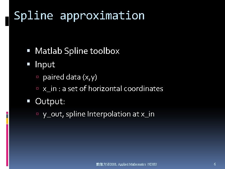
Spline approximation Matlab Spline toolbox Input paired data (x, y) x_in : a set of horizontal coordinates Output: y_out, spline Interpolation at x_in 數值方法 2008, Applied Mathematics NDHU 6

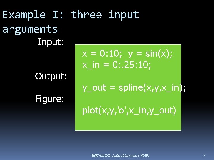
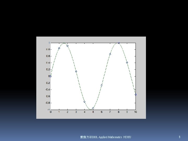
Example I: three input arguments Input: Output: Figure: x = 0: 10; y = sin(x); x_in = 0: . 25: 10; y_out = spline(x, y, x_in); plot(x, y, 'o', x_in, y_out) 數值方法 2008, Applied Mathematics NDHU 7

數值方法 2008, Applied Mathematics NDHU 8

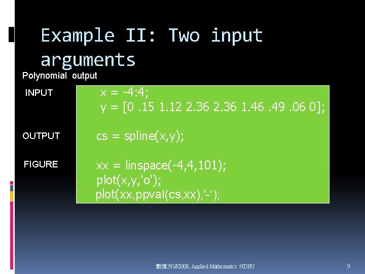
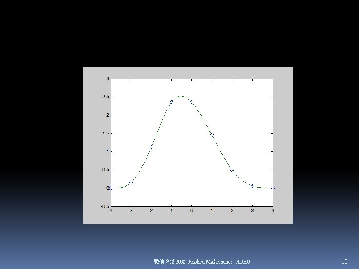
Example II: Two input arguments Polynomial output INPUT x = -4: 4; y = [0. 15 1. 12 2. 36 1. 46. 49. 06 0]; OUTPUT cs = spline(x, y); FIGURE xx = linspace(-4, 4, 101); plot(x, y, 'o'); plot(xx, ppval(cs, xx), '-‘); 數值方法 2008, Applied Mathematics NDHU 9

數值方法 2008, Applied Mathematics NDHU 10

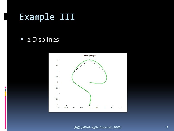
Example III 2 D splines 數值方法 2008, Applied Mathematics NDHU 11

2 -D spline demo_2 d_spline. m 數值方法 2008, Applied Mathematics NDHU 12

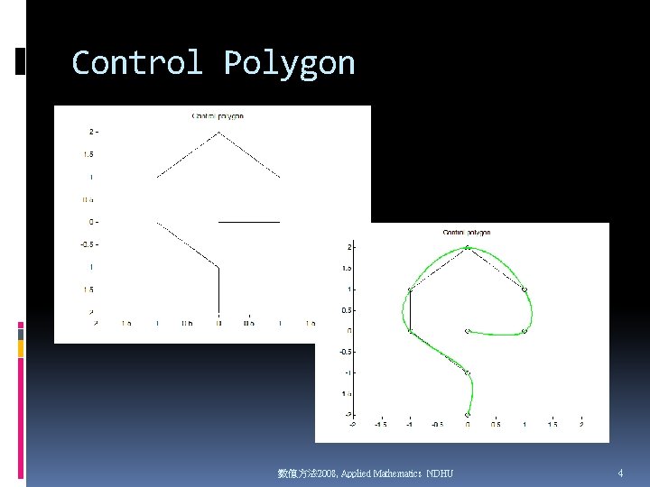
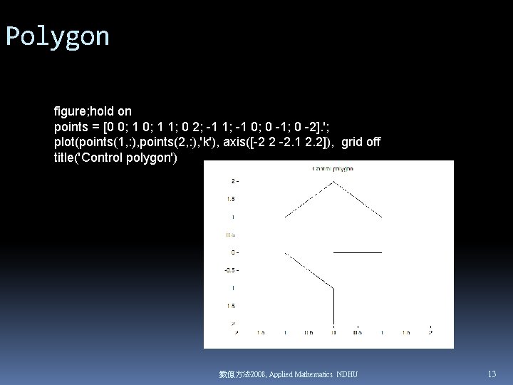
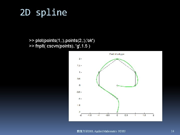
Polygon figure; hold on points = [0 0; 1 1; 0 2; -1 1; -1 0; 0 -1; 0 -2]. '; plot(points(1, : ), points(2, : ), 'k'), axis([-2 2 -2. 1 2. 2]), grid off title('Control polygon') 數值方法 2008, Applied Mathematics NDHU 13

2 D spline >> plot(points(1, : ), points(2, : ), 'ok') >> fnplt( cscvn(points), 'g', 1. 5 ) 數值方法 2008, Applied Mathematics NDHU 14

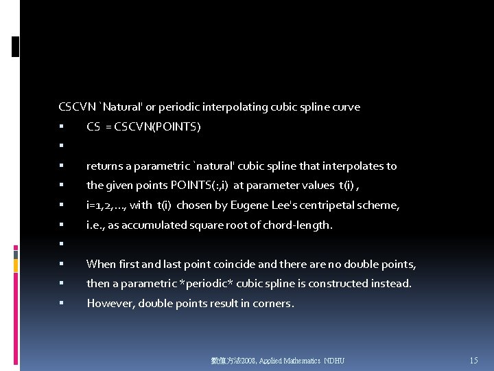
CSCVN `Natural' or periodic interpolating cubic spline curve CS = CSCVN(POINTS) returns a parametric `natural' cubic spline that interpolates to the given points POINTS(: , i) at parameter values t(i) , i=1, 2, . . . , with t(i) chosen by Eugene Lee's centripetal scheme, i. e. , as accumulated square root of chord-length. When first and last point coincide and there are no double points, then a parametric *periodic* cubic spline is constructed instead. However, double points result in corners. 數值方法 2008, Applied Mathematics NDHU 15

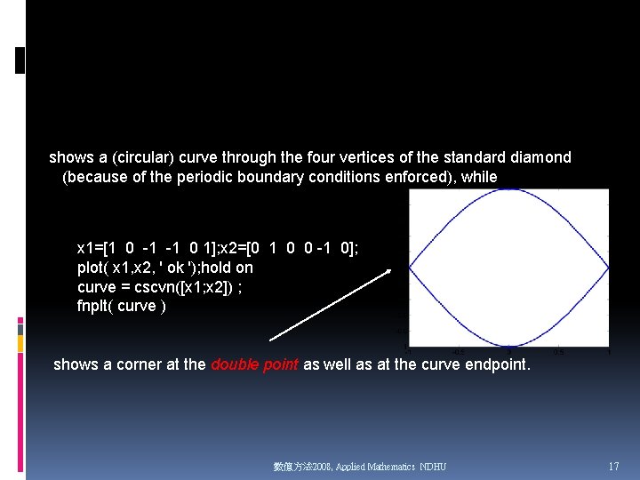
For example, x 1=[1 0 -1 0 1]; x 2=[0 1 0 -1 0]; plot( x 1, x 2, ' ok '); hold on curve = cscvn([x 1; x 2]) ; fnplt( curve ) 數值方法 2008, Applied Mathematics NDHU 16

shows a (circular) curve through the four vertices of the standard diamond (because of the periodic boundary conditions enforced), while x 1=[1 0 -1 -1 0 1]; x 2=[0 1 0 0 -1 0]; plot( x 1, x 2, ' ok '); hold on curve = cscvn([x 1; x 2]) ; fnplt( curve ) shows a corner at the double point as well as at the curve endpoint. 數值方法 2008, Applied Mathematics NDHU 17

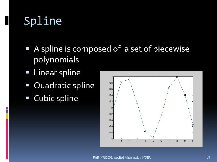
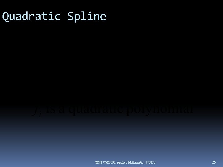
Spline A spline is composed of a set of piecewise polynomials Linear spline Quadratic spline Cubic spline 數值方法 2008, Applied Mathematics NDHU 18

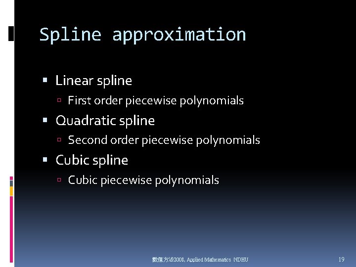
Spline approximation Linear spline First order piecewise polynomials Quadratic spline Second order piecewise polynomials Cubic spline Cubic piecewise polynomials 數值方法 2008, Applied Mathematics NDHU 19

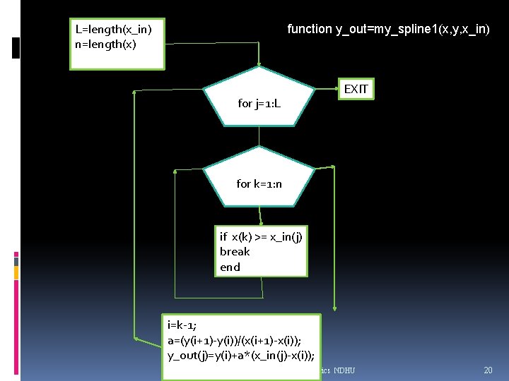
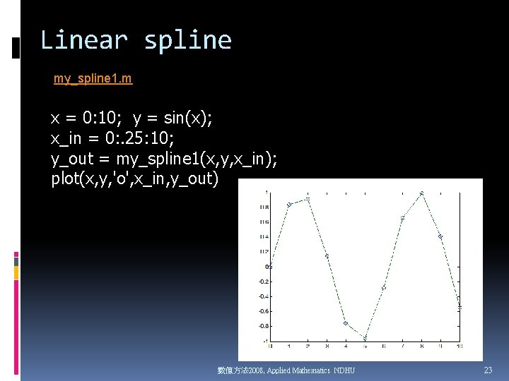
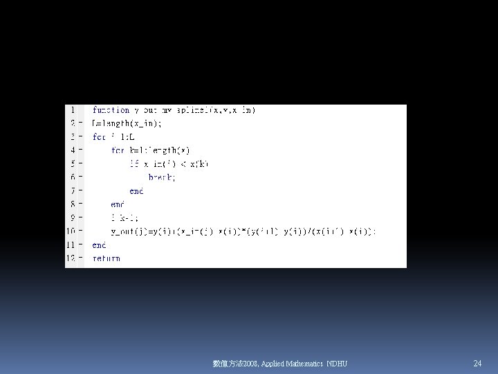
L=length(x_in) n=length(x) function y_out=my_spline 1(x, y, x_in) for j=1: L EXIT for k=1: n if x(k) >= x_in(j) break end i=k-1; a=(y(i+1)-y(i))/(x(i+1)-x(i)); y_out(j)=y(i)+a*(x_in(j)-x(i)); 數值方法 2008, Applied Mathematics NDHU 20

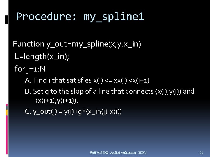
Procedure: my_spline 1 Function y_out=my_spline(x, y, x_in) L=length(x_in); for j=1: N A. Find i that satisfies x(i) <= xx(i) <x(i+1) B. Set g to the slop of a line that connects (x(i), y(i)) and (x(i+1), y(i+1)). C. y_out(j) = y(i)+g*(x_in(j)-x(i)) 數值方法 2008, Applied Mathematics NDHU 21

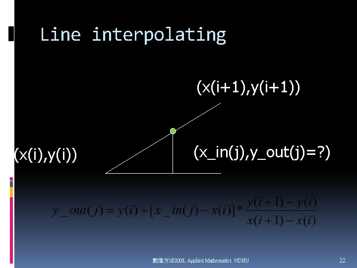
Line interpolating (x(i+1), y(i+1)) (x(i), y(i)) (x_in(j), y_out(j)=? ) 數值方法 2008, Applied Mathematics NDHU 22

Linear spline my_spline 1. m x = 0: 10; y = sin(x); x_in = 0: . 25: 10; y_out = my_spline 1(x, y, x_in); plot(x, y, 'o', x_in, y_out) 數值方法 2008, Applied Mathematics NDHU 23

數值方法 2008, Applied Mathematics NDHU 24

Quadratic Spline 數值方法 2008, Applied Mathematics NDHU 25

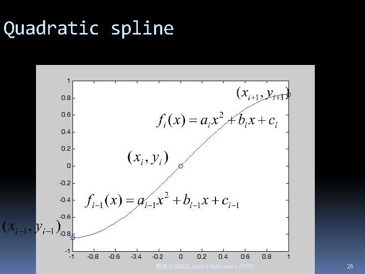
Quadratic spline 數值方法 2008, Applied Mathematics NDHU 26

Quadratic splines Quadratic spline interpolation Determine all fi 數值方法 2008, Applied Mathematics NDHU 27

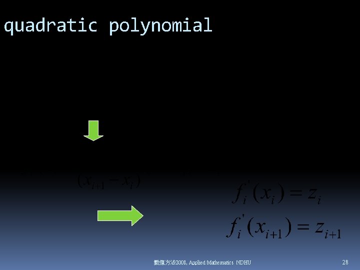
quadratic polynomial 數值方法 2008, Applied Mathematics NDHU 28

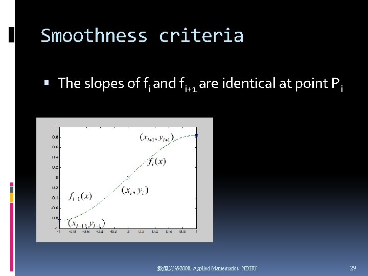
Smoothness criteria The slopes of fi and fi+1 are identical at point Pi 數值方法 2008, Applied Mathematics NDHU 29

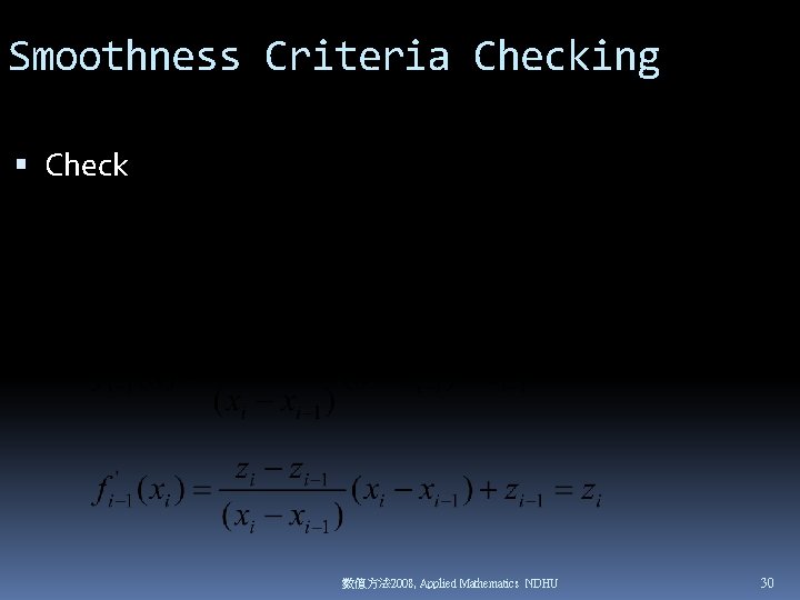
Smoothness Criteria Checking Check 數值方法 2008, Applied Mathematics NDHU 30

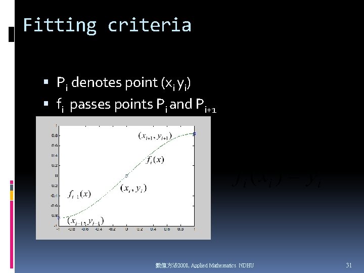
Fitting criteria Pi denotes point (xi yi) fi passes points Pi and Pi+1 數值方法 2008, Applied Mathematics NDHU 31

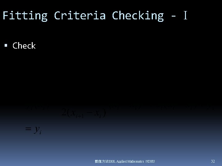
Fitting Criteria Checking - I Check 數值方法 2008, Applied Mathematics NDHU 32

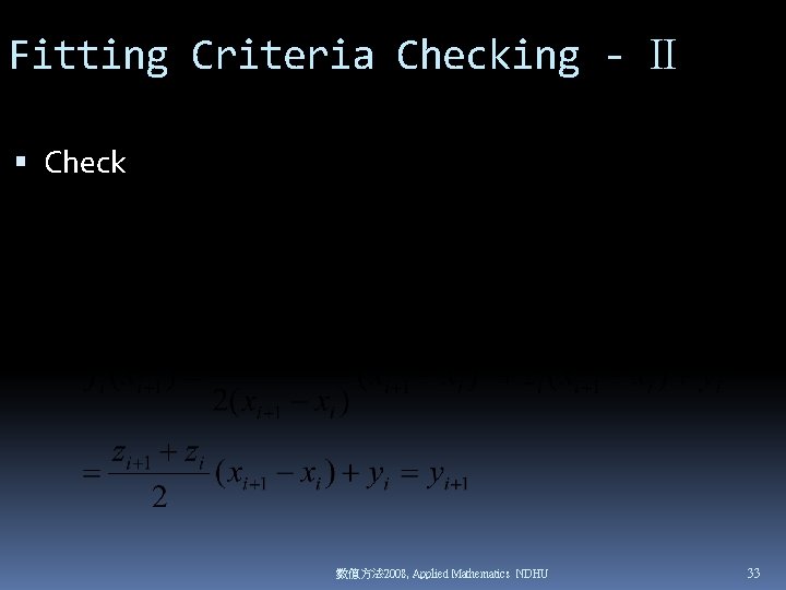
Fitting Criteria Checking - II Check 數值方法 2008, Applied Mathematics NDHU 33

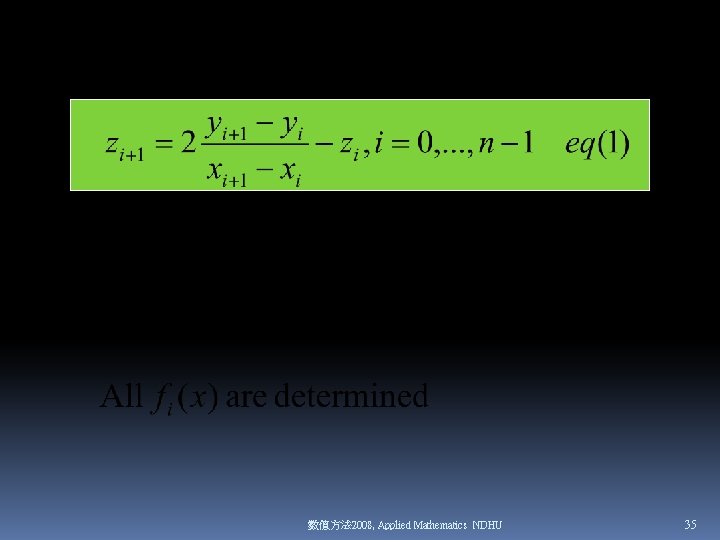
Recurrence relations 數值方法 2008, Applied Mathematics NDHU 34

數值方法 2008, Applied Mathematics NDHU 35

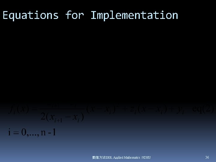
Equations for Implementation 數值方法 2008, Applied Mathematics NDHU 36

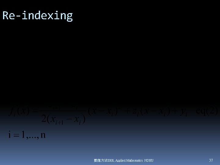
Re-indexing 數值方法 2008, Applied Mathematics NDHU 37

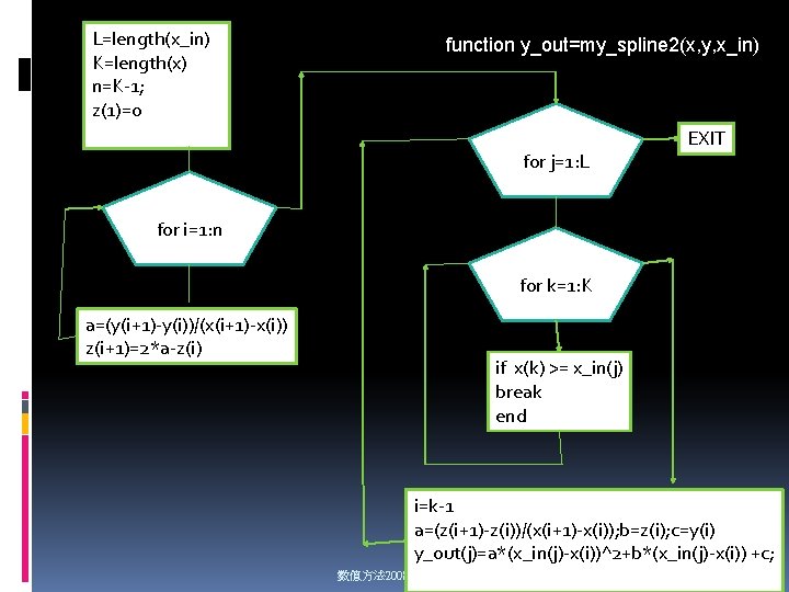
L=length(x_in) K=length(x) n=K-1; z(1)=0 function y_out=my_spline 2(x, y, x_in) for j=1: L EXIT for i=1: n for k=1: K a=(y(i+1)-y(i))/(x(i+1)-x(i)) z(i+1)=2*a-z(i) if x(k) >= x_in(j) break end i=k-1 a=(z(i+1)-z(i))/(x(i+1)-x(i)); b=z(i); c=y(i) y_out(j)=a*(x_in(j)-x(i))^2+b*(x_in(j)-x(i)) +c; 數值方法 2008, Applied Mathematics NDHU 38

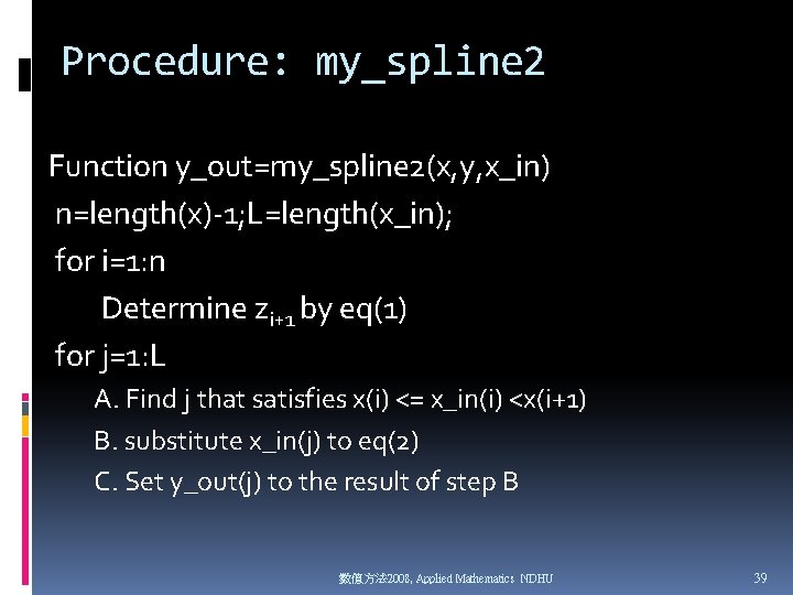
Procedure: my_spline 2 Function y_out=my_spline 2(x, y, x_in) n=length(x)-1; L=length(x_in); for i=1: n Determine zi+1 by eq(1) for j=1: L A. Find j that satisfies x(i) <= x_in(i) <x(i+1) B. substitute x_in(j) to eq(2) C. Set y_out(j) to the result of step B 數值方法 2008, Applied Mathematics NDHU 39

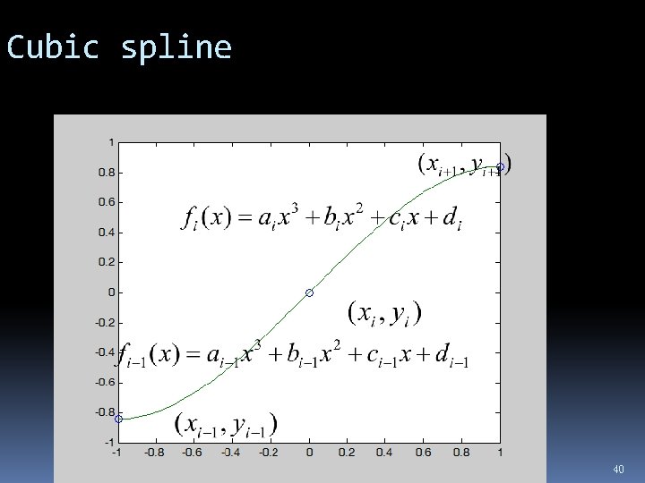
Cubic spline 數值方法 2008, Applied Mathematics NDHU 40

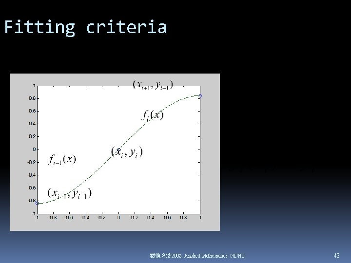
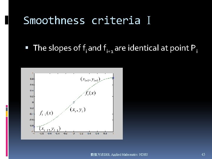
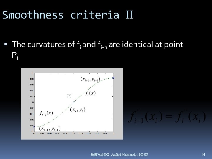
Criteria of cubic spline Fitting criteria First order smoothness criteria Second order smoothness criteria 數值方法 2008, Applied Mathematics NDHU 41

Fitting criteria 數值方法 2008, Applied Mathematics NDHU 42

Smoothness criteria I The slopes of fi and fi+1 are identical at point Pi 數值方法 2008, Applied Mathematics NDHU 43

Smoothness criteria II The curvatures of fi and fi+1 are identical at point Pi Pi 數值方法 2008, Applied Mathematics NDHU 44

Exercise Draw a flow chart to illustrate linear spline interpolation Implement the flow chart by matlab codes Give examples to test your matlab codes 數值方法 2008, Applied Mathematics NDHU 45

Exercise Draw a flow chart to illustrate quadratic spline interpolation Implement the flow chart by matlab codes Give examples to test your matlab codes 數值方法 2008, Applied Mathematics NDHU 46