Splay Tree Algorithm Mingda Zhao CSC 252 Algorithms

Splay Tree Algorithm Mingda Zhao CSC 252 Algorithms Smith College Fall, 2000

Contents What is Splay Tree? Splaying: zig-zig; zig-zag; zig. Rules: search; insertion; deletion. Complexity analysis. Implementation. Demos Conclusion References

What is Splay Tree? A balanced search tree data structure NIST Definition: A binary search tree in which operations that access nodes restructure the tree. Goodrich: A splay tree is a binary search tree T. The only tool used to maintain balance in T is the splaying step done after every search, insertion, and deletion in T. Kingston: A binary tee with splaying.

Splaying Left and right rotation Move-to-root operation Zig-zig Zig-zag Zig Comparing move-to-root and splaying Example of splaying a node

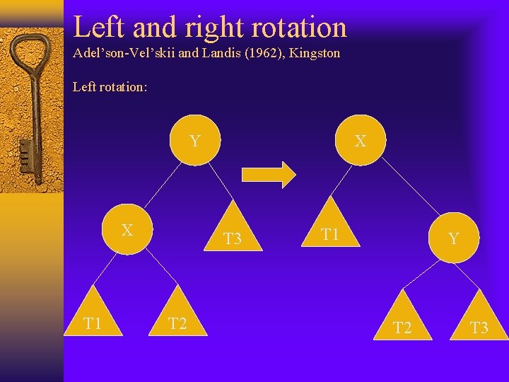
Left and right rotation Adel’son-Vel’skii and Landis (1962), Kingston Left rotation: Y X T 1 X T 3 T 2 T 1 Y T 2 T 3

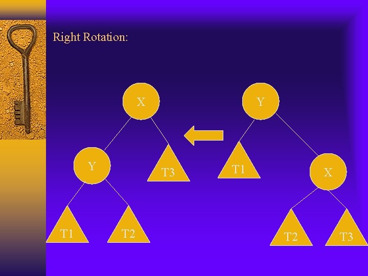
Right Rotation: X Y T 1 Y T 3 T 2 T 1 X T 2 T 3

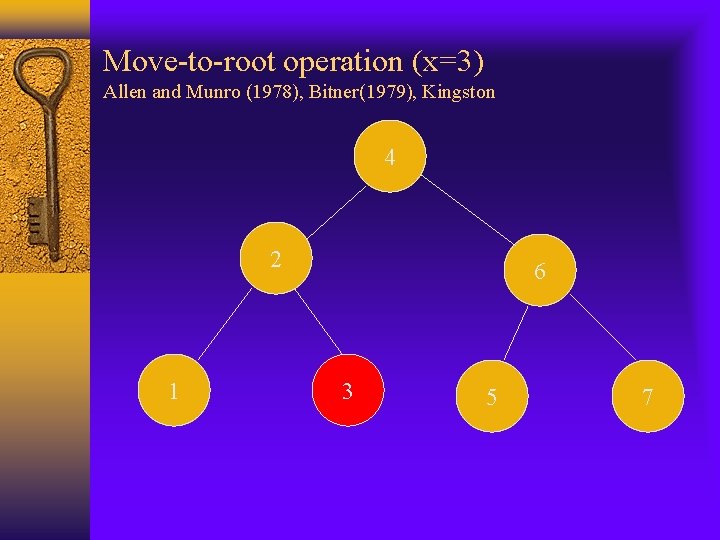
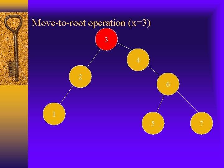
Move-to-root operation (x=3) Allen and Munro (1978), Bitner(1979), Kingston 4 2 1 6 3 5 7

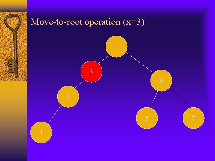
Move-to-root operation (x=3) 4 3 6 2 5 1 7

Move-to-root operation (x=3) 3 4 2 6 1 5 7

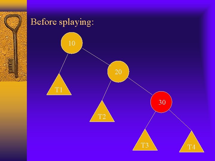
Zig-zig splaying The node x and its parent y are both left children or both right children. We replace z by x, making y a child of x and z a child of y, while maintaining the inorder relationships of the nodes in tree T. Example: x is 30, y is 20, z is 10

Before splaying: 10 20 T 1 30 T 2 T 3 T 4

After splaying: 30 20 T 4 10 T 3 T 1 T 2

Zig-zag splaying One of x and y is a left child and the other is a right child. We replace z by x and make x have nodes y and z as its children, while maintaining the inorder relationships of the nodes in tree T. Example: z is 10, y is 30, x is 20

Before splaying: 10 30 T 1 20 T 4 T 2 T 3

After splaying: 20 10 T 1 30 T 2 T 3 T 4

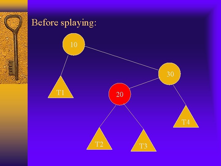
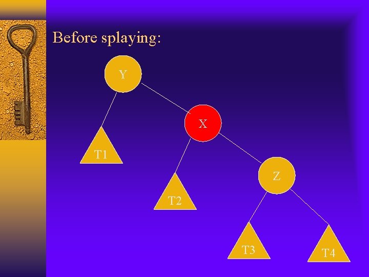
Zig splaying X doesn’t have a grand parent(or the grandparent is not considered) We rotate x over y, making x’s children be the node y and one of x’s former children u, so as to maintain the relative inorder relationships of the nodes in tree T. Example: x is 20, y is 10, u is 30

Before splaying: 10 20 T 1 30 T 2 T 3 T 4

After splaying: 20 10 T 1 30 T 2 T 3 T 4

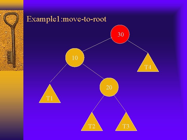
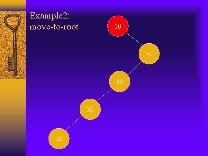
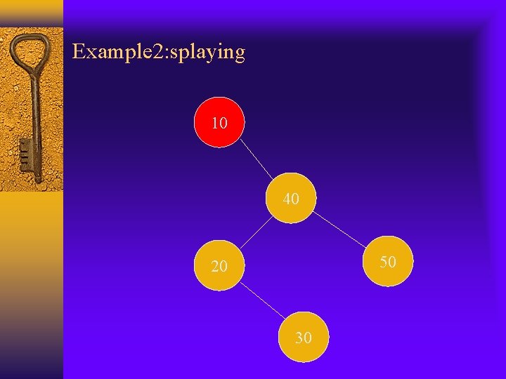
Move-to-root vs. splaying Move-to-root should improve the performance of the BST when there is locality of references in the operation sequence, but it is not ideal. The example we use before, the result is not balanced even the original tree was. Splaying also moves the subtrees of node x(which is being splayed) up 1 level, but move-to-root usually leaves one subtree at its original level. Example:

Example 1: original tree 10 20 T 1 30 T 2 T 3 T 4

Example 1: move-to-root 30 10 T 4 20 T 1 T 2 T 3

Example 1: splaying 30 20 T 4 10 T 3 T 1 T 2

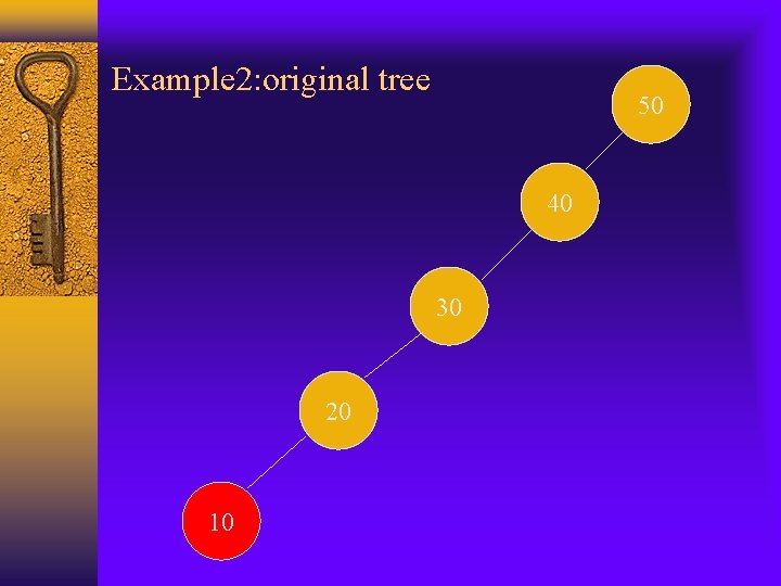
Example 2: original tree 50 40 30 20 10

Example 2: move-to-root 10 50 40 30 20

Example 2: splaying 10 40 50 20 30

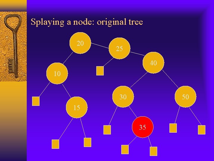
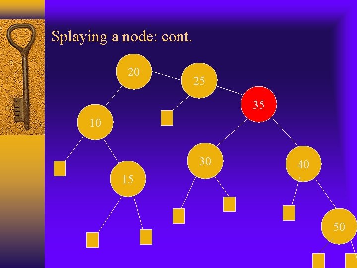
Splaying a node: original tree 20 25 40 10 30 50 15 35

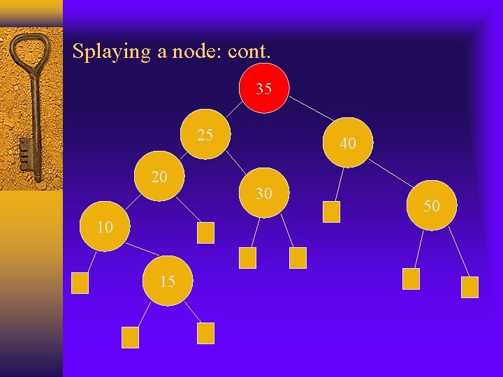
Splaying a node: cont. 20 25 35 10 30 40 15 50

Splaying a node: cont. 35 25 20 10 15 40 30 50

Rules of splaying: Search When search for key I, if I is found at node x, we splay x. If not successful, we splay the parent of the external node at which the search terminates unsuccessfully. (null node) Example: see above slides, it can be for successfully searched I=35 or unsuccessfully searched say I=38.

Rules of splaying: insertion When inserting a key I, we splay the newly created internal node where I was inserted. Example:

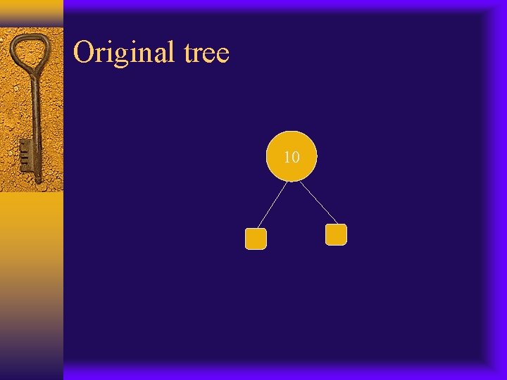
Original tree 10

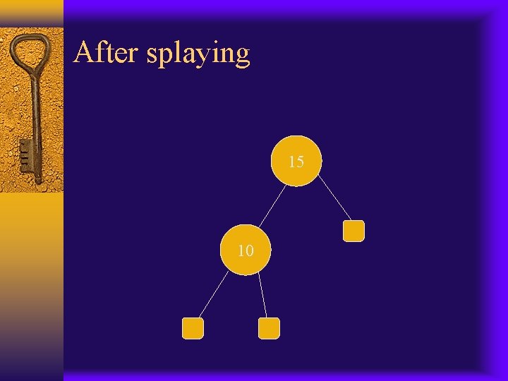
After insert key 15 10 15

After splaying 15 10

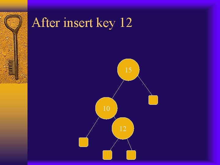
After insert key 12 15 10 12

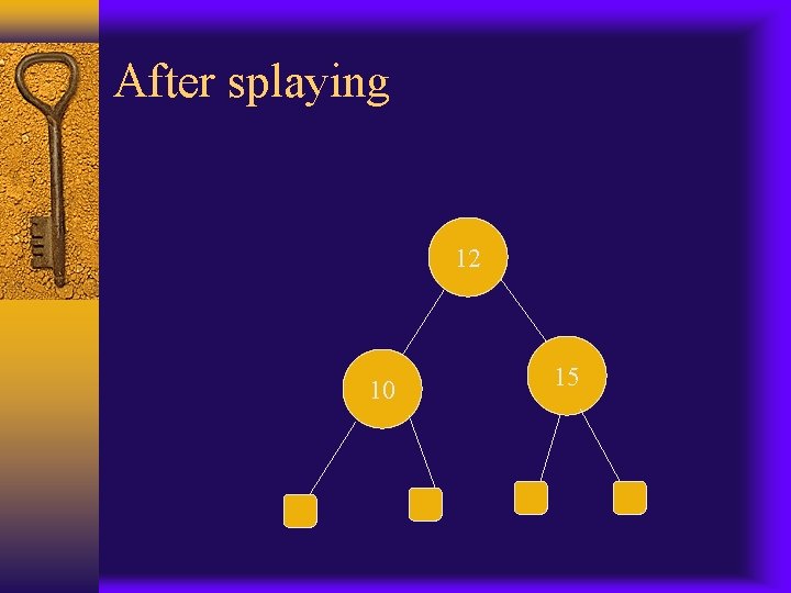
After splaying 12 10 15

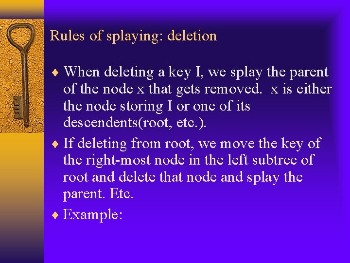
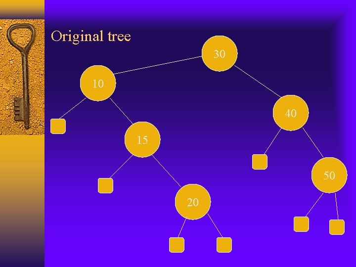
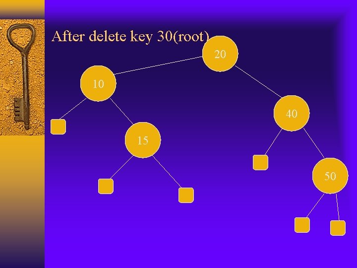
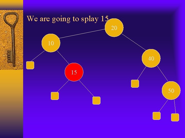
Rules of splaying: deletion When deleting a key I, we splay the parent of the node x that gets removed. x is either the node storing I or one of its descendents(root, etc. ). If deleting from root, we move the key of the right-most node in the left subtree of root and delete that node and splay the parent. Etc. Example:

Original tree 30 10 40 15 50 20

After delete key 30(root) 20 10 40 15 50

We are going to splay 15 20 10 40 15 50

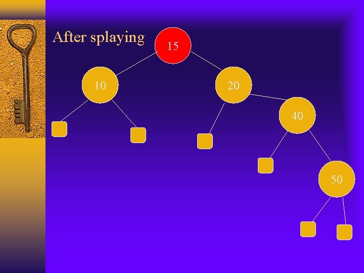
After splaying 10 15 20 40 50

Complexity Worst case: O(n), all nodes are on one side of the subtree. (In fact, it is (n). ) Amortized Analysis: We will only consider the splaying time, since the time for perform search, insertion or deletion is proportional to the time for the splaying they are associated with.

Amortized analysis Let n(v) = the number of nodes in the subtree rooted at v Let r(v) = log(n(v)), rank. Let r’(v) be the rank of node v after splaying. If a>0, b>0, and c>a+b, then log a + log b <= 2 log c – 2 *Search the key takes d time, d = depth of the node before splaying.

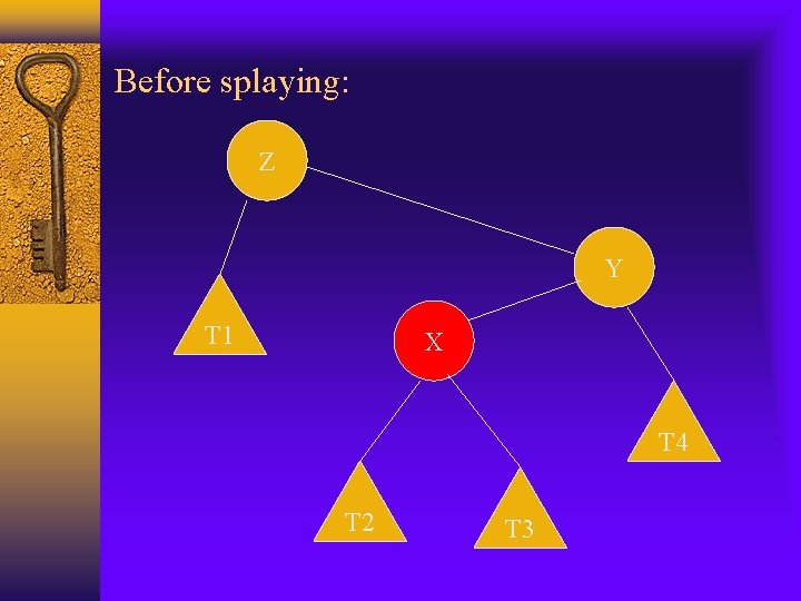
Before splaying: Z Y T 1 X T 2 T 3 T 4

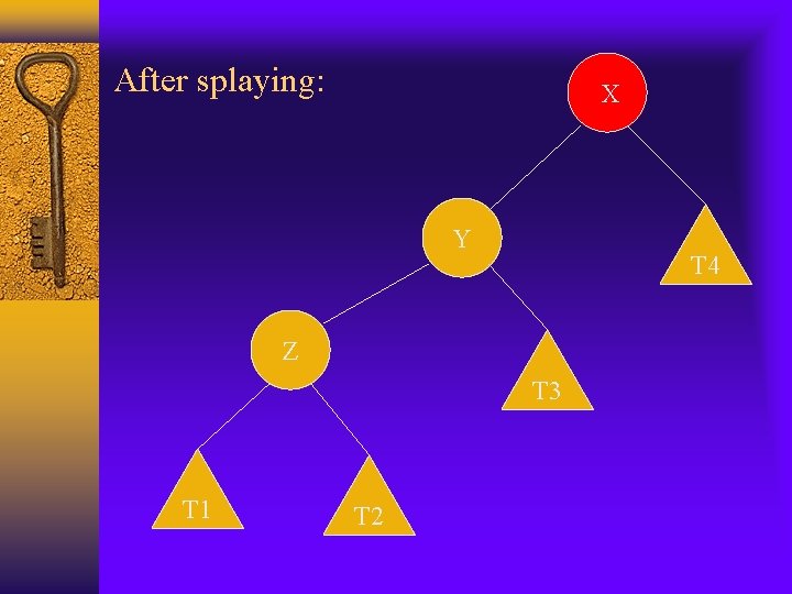
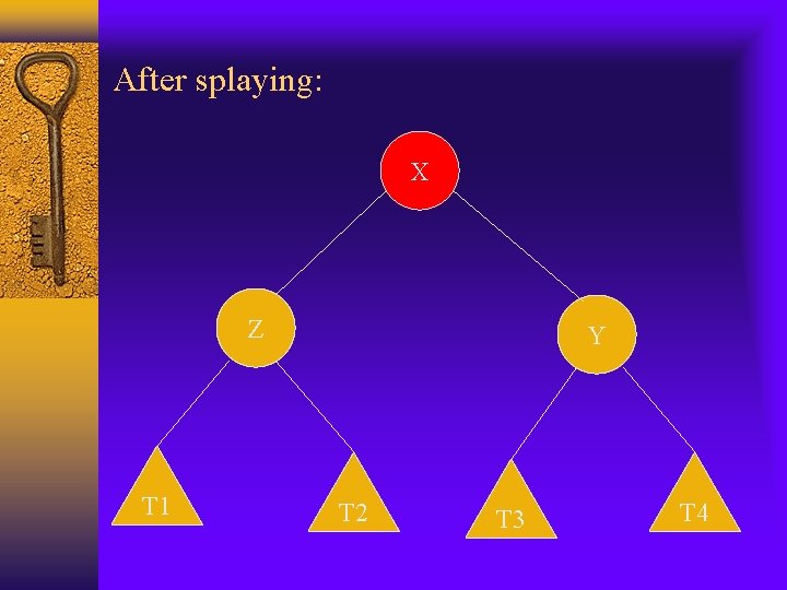
After splaying: X Y T 4 Z T 3 T 1 T 2

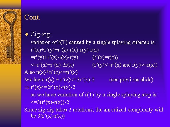
Cont. Zig-zig: variation of r(T) caused by a single splaying substep is: r’(x)+r’(y)+r’(z)-r(x)-r(y)-r(z) =r’(y)+r’(z)-r(x)-r(y) (r’(x)=r(z)) <=r’(x)+r’(z)-2 r(x) (r’(y)<=r’(x) and r(y)>=r(x)) Also n(x)+n’(z)<=n’(x) We have r(x) + r’(z)<=2 r’(x)-2 (see previous slide) r’(z)<=2 r’(x)-r(x)-2 so we have variation of r(T) by a single splaying step is: <=3(r’(x)-r(x))-2 Since zig-zig takes 2 rotations, the amortized complexity will be 3(r’(x)-r(x))

Before splaying: Z Y T 1 X T 4 T 2 T 3

After splaying: X Z T 1 Y T 2 T 3 T 4

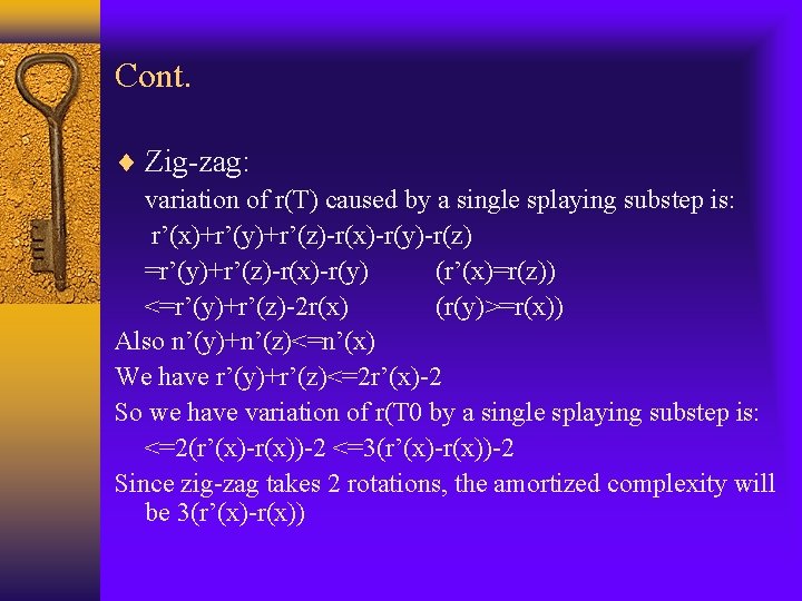
Cont. Zig-zag: variation of r(T) caused by a single splaying substep is: r’(x)+r’(y)+r’(z)-r(x)-r(y)-r(z) =r’(y)+r’(z)-r(x)-r(y) (r’(x)=r(z)) <=r’(y)+r’(z)-2 r(x) (r(y)>=r(x)) Also n’(y)+n’(z)<=n’(x) We have r’(y)+r’(z)<=2 r’(x)-2 So we have variation of r(T 0 by a single splaying substep is: <=2(r’(x)-r(x))-2 <=3(r’(x)-r(x))-2 Since zig-zag takes 2 rotations, the amortized complexity will be 3(r’(x)-r(x))

Before splaying: Y X T 1 Z T 2 T 3 T 4

After splaying: X Y T 1 Z T 2 T 3 T 4

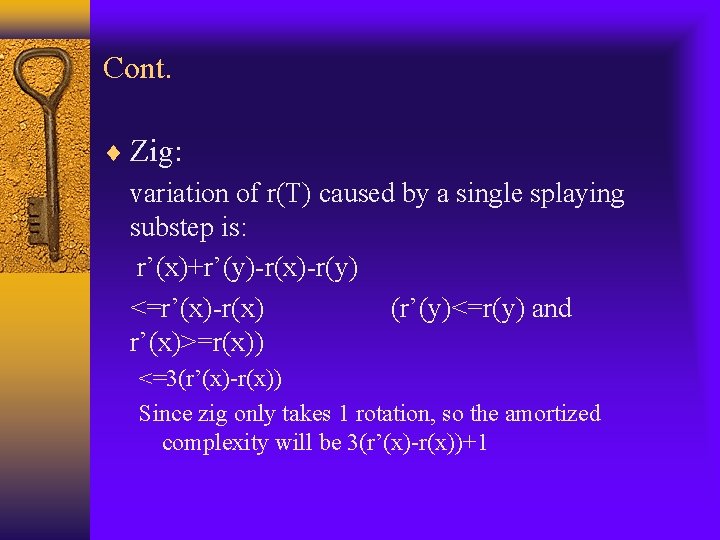
Cont. Zig: variation of r(T) caused by a single splaying substep is: r’(x)+r’(y)-r(x)-r(y) <=r’(x)-r(x) (r’(y)<=r(y) and r’(x)>=r(x)) <=3(r’(x)-r(x)) Since zig only takes 1 rotation, so the amortized complexity will be 3(r’(x)-r(x))+1

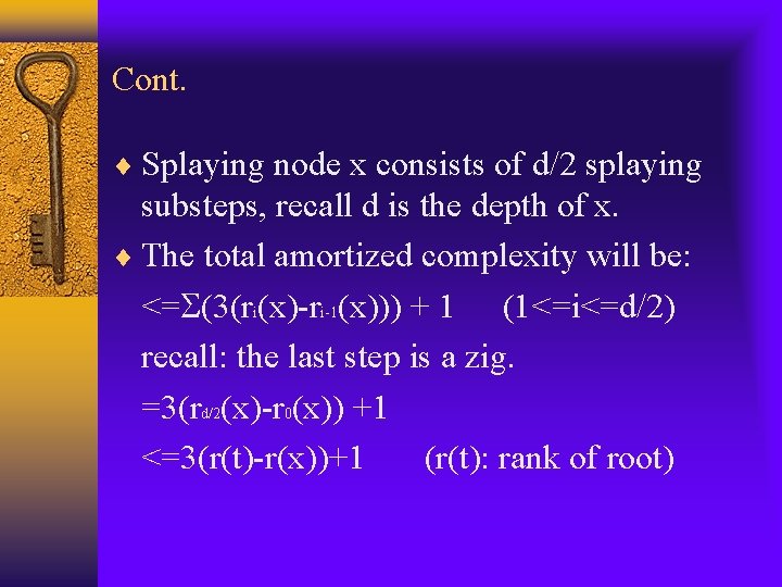
Cont. Splaying node x consists of d/2 splaying substeps, recall d is the depth of x. The total amortized complexity will be: <= (3(ri(x)-ri-1(x))) + 1 (1<=i<=d/2) recall: the last step is a zig. =3(rd/2(x)-r 0(x)) +1 <=3(r(t)-r(x))+1 (r(t): rank of root)

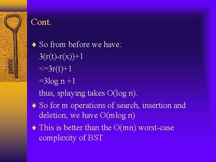
Cont. So from before we have: 3(r(t)-r(x))+1 <=3 r(t)+1 =3 log n +1 thus, splaying takes O(log n). So for m operations of search, insertion and deletion, we have O(mlog n) This is better than the O(mn) worst-case complexity of BST

Implementation LEDA ? Java implementation: Splay. Tree. java and etc from previous files(? ) Modified print. Tree() to track level and child identity, add a small testing part.

Demos A Demo written in Perl, it has some small bugs http: //bobo. link. cs. cmu. edu/cgibin/splay-cgi. pl An animation java applet: http: //www. cs. technion. ac. il/~itai/ds 2/frame splay/splay. html

Conclusion A balanced binary search tree. Doesn’t need any extra information to be stored in the node, ie color, level, etc. Balanced in an amortized sense. Running time is O(mlog n) for m operations Can be adapted to the ways in which items are being accessed in a dictionary to achieve faster running times for the frequently accessed items. (O(1), AVL is about O(log n), etc. )

References Data Structure and Algorithms in Java, Michael T. Good. Rich. Algorithms and Data Structures, Jeffrey H Kingston http: //www. cs. mcgill. ca/~rsinge/web 251. html http: //hissa. nist. gov/dads/HTML/splaytree. html NIST Data Strucrues and Problem Solving with C++, Frank M. Carrano. Source code: http: //www. aw. com/cseng/ http: //www. labmed. umn. edu/~michael/Splay/readme. html