Splay tree 2 3 4 tree Marko Berezovsk

Splay tree, 2 -3 -4 tree Marko Berezovský Radek Mařík PAL 2012 p 2<1 Hi! To read ? / x+y x--y [1] Weiss M. A. , Data Structures and Algorithm Analysis in C++, 3 rd Ed. , Addison Wesley, § 4. 5, pp. 149 -58. [2] Daniel D. Sleator and Robert E. Tarjan, "Self-Adjusting Binary Search Trees", Journal of the ACM 32 (3), 1985, pp. 652 -86. [3] Ben Pfaff: Performance Analysis of BSTs in System Software, 2004, Stanford University, Department of Computer Science, http: //benpfaff. org/papers/libavl. pdf See also PAL webpage for references Pokročilá Algoritmizace, A 4 M 33 PAL, ZS 2012/2013, FEL ČVUT, 12/14

Splay Tree - Description Basic idea AVL trees and red-black trees are binary search trees with logarithmic height. This ensures all operations are O(ln(n)) An alternative idea is to make use of an old maxim: Data that has been recently accessed is more likely to be accessed again in the near future. Accessed nodes are splayed ( = moved by one or more rotations) to the root of the tree: Find the node like in a BST and then splay it to the root. Insert: Insert the node like in a BST and then splay it to the root. Delete: Splay the node to the root and then delete it like in a BST. Invented in 1985 by Daniel Dominic Sleator and Robert Endre Tarjan. Pokročilá Algoritmizace, A 4 M 33 PAL, ZS 2012/2013, FEL ČVUT, 12/14 1

Splay Tree - Description Properties overview Splay tree - A binary search tree. - No additional tree shape description (no additional memory!) is used. - Each node access or insertion splays that node to the root. - Rotations are zig, zig-zig and zig-zag, based on BST single rotation. - All operations run times are O(n), as the tree height can be (n). - Amortized run times of all operations are O(ln(n)). Pokročilá Algoritmizace, A 4 M 33 PAL, ZS 2012/2013, FEL ČVUT, 12/14 2

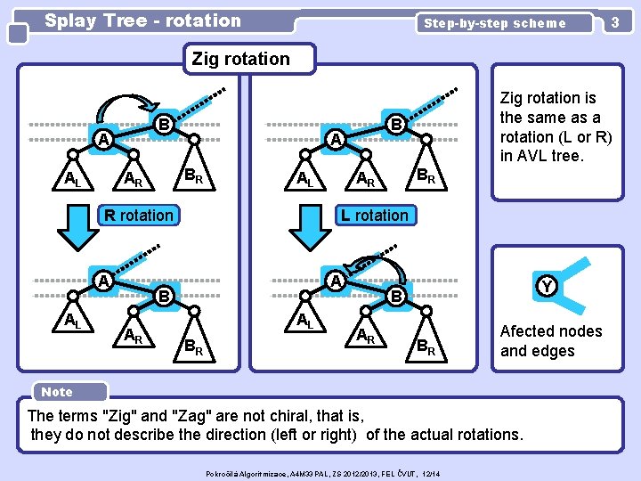
Splay Tree - rotation Step-by-step scheme 3 Zig rotation B A AL AL R rotation A AL BR AR L rotation A B AR B A BR AR Zig rotation is the same as a rotation (L or R) in AVL tree. AL BR Y B AR BR Afected nodes and edges Note The terms "Zig" and "Zag" are not chiral, that is, they do not describe the direction (left or right) of the actual rotations. Pokročilá Algoritmizace, A 4 M 33 PAL, ZS 2012/2013, FEL ČVUT, 12/14

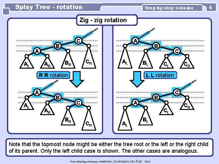
Splay Tree - rotation Step-by-step scheme Zig - zig rotation B A AL C CR BR AR A AL BL R R rotation A AL B C CL CR L L rotation B C C B A AR CL BR CR AL CR BL Note that the topmost node might be either the tree root or the left or the right child of its parent. Only the left child case is shown. The other cases are analogous. Pokročilá Algoritmizace, A 4 M 33 PAL, ZS 2012/2013, FEL ČVUT, 12/14 4

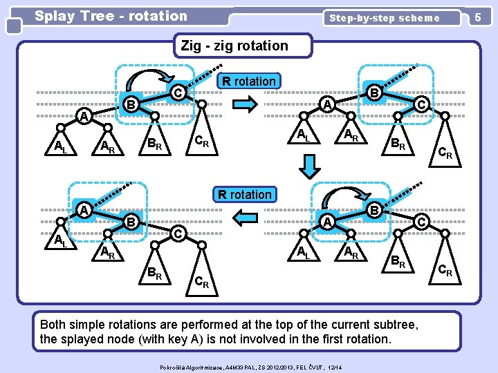
Splay Tree - rotation Step-by-step scheme Zig - zig rotation AL C B A AL CR BR AR R rotation AR C BR CR R rotation A AL B A C AR AL BR B AR C BR CR Both simple rotations are performed at the top of the current subtree, the splayed node (with key A) is not involved in the first rotation. Pokročilá Algoritmizace, A 4 M 33 PAL, ZS 2012/2013, FEL ČVUT, 12/14 CR 5

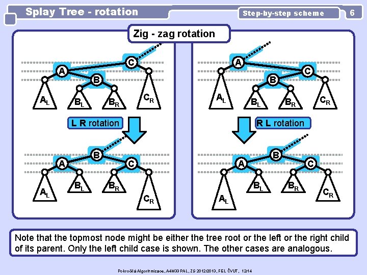
Splay Tree - rotation Step-by-step scheme Zig - zag rotation C A AL A B BL B CR BR AL BL L R rotation B A AL BL C CR BR R L rotation C B A BR BL CR AL C BR CR Note that the topmost node might be either the tree root or the left or the right child of its parent. Only the left child case is shown. The other cases are analogous. Pokročilá Algoritmizace, A 4 M 33 PAL, ZS 2012/2013, FEL ČVUT, 12/14 6

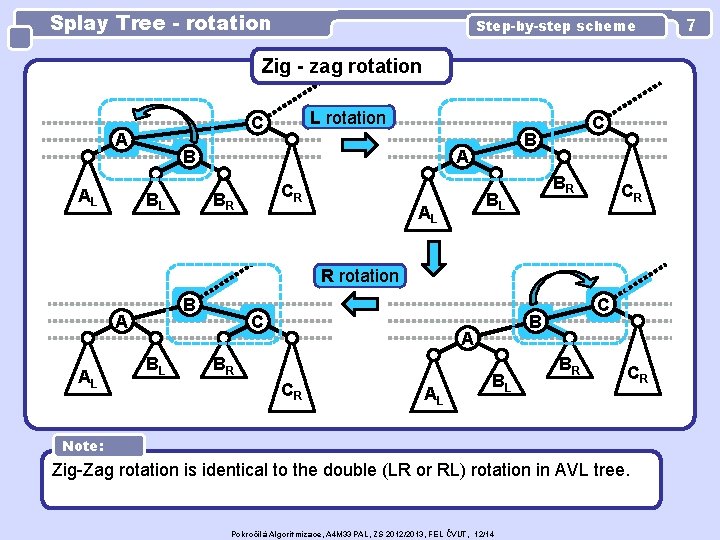
Splay Tree - rotation Step-by-step scheme Zig - zag rotation A AL L rotation C B BL B A CR BR BR BL AL C CR R rotation B A AL BL C B A BR CR AL C BL BR CR Note: Zig-Zag rotation is identical to the double (LR or RL) rotation in AVL tree. Pokročilá Algoritmizace, A 4 M 33 PAL, ZS 2012/2013, FEL ČVUT, 12/14 7

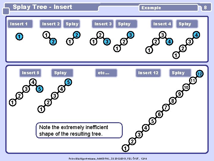
Splay Tree - Insert 1 Insert 2 Splay 1 1 Insert 3 2 2 1 Splay 2 1 Insert 4 3 3 Splay 4 3 Splay 3 2 4 2 1 Insert 5 8 Example 4 3 2 1 etc. . . 1 Insert 12 Splay 11 5 5 10 4 2 9 3 1 12 8 2 7 1 6 5 Note the extremely inefficient shape of the resulting tree. 4 3 2 1 Pokročilá Algoritmizace, A 4 M 33 PAL, ZS 2012/2013, FEL ČVUT, 12/14

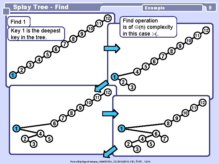
Splay Tree - Find 12 Find 1 1 4 3 2 Find operation is of (n) complexity in this case : -(. 11 Key 1 is the deepest key in the tree. 5 6 7 9 Example 8 9 10 1 5 4 2 6 12 11 9 8 7 10 3 12 11 6 1 2 4 3 5 7 8 9 10 12 11 8 1 2 4 3 6 5 Pokročilá Algoritmizace, A 4 M 33 PAL, ZS 2012/2013, FEL ČVUT, 12/14 7 9 10

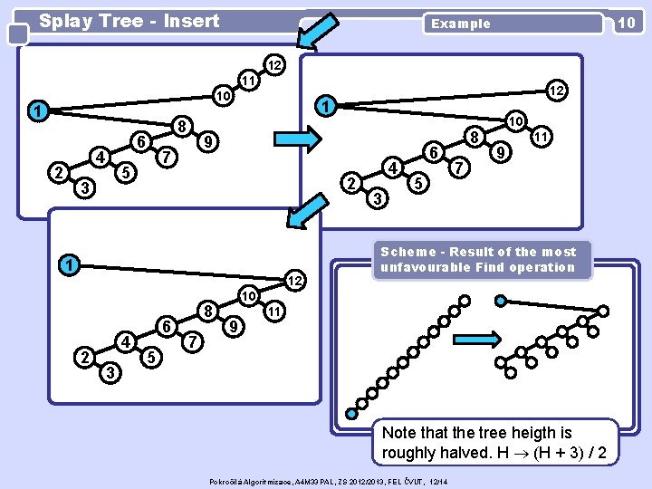
Splay Tree - Insert 10 Example 12 11 10 1 6 4 2 8 3 1 9 7 5 2 1 12 2 4 3 12 6 5 8 7 4 3 6 5 8 7 10 9 11 Scheme - Result of the most unfavourable Find operation 10 9 11 Note that the tree heigth is roughly halved. H (H + 3) / 2 Pokročilá Algoritmizace, A 4 M 33 PAL, ZS 2012/2013, FEL ČVUT, 12/14

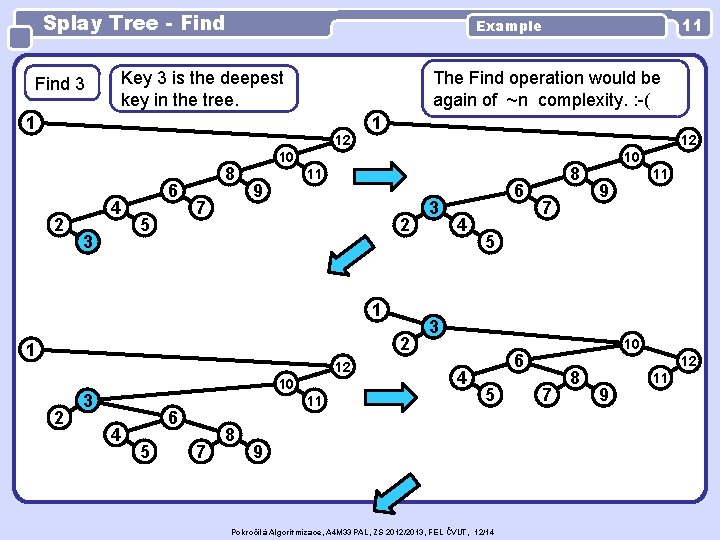
Splay Tree - Find 3 The Find operation would be again of ~n complexity. : -( Key 3 is the deepest key in the tree. 1 12 2 4 3 6 5 8 7 1 12 10 11 9 2 1 12 2 10 3 4 11 6 5 7 11 Example 8 3 6 4 8 7 10 9 5 3 4 11 10 6 5 9 Pokročilá Algoritmizace, A 4 M 33 PAL, ZS 2012/2013, FEL ČVUT, 12/14 7 8 12 9 11

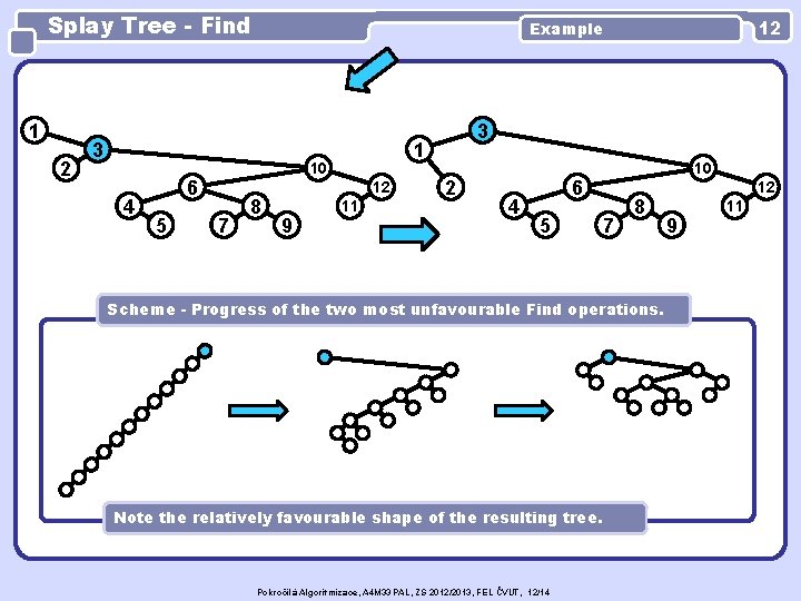
Splay Tree - Find 1 2 3 4 5 7 8 12 9 3 1 10 6 12 Example 11 2 4 10 6 5 7 8 Scheme - Progress of the two most unfavourable Find operations. Note the relatively favourable shape of the resulting tree. Pokročilá Algoritmizace, A 4 M 33 PAL, ZS 2012/2013, FEL ČVUT, 12/14 12 9 11

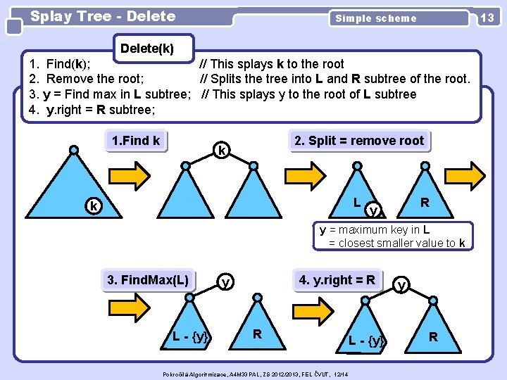
Splay Tree - Delete 13 Simple scheme Delete(k) 1. Find(k); // This splays k to the root 2. Remove the root; // Splits the tree into L and R subtree of the root. 3. y = Find max in L subtree; // This splays y to the root of L subtree 4. y. right = R subtree; 1. Find k 2. Split = remove root k L k R y y = maximum key in L = closest smaller value to k 3. Find. Max(L) L - {y} 4. y. right = R y R Pokročilá Algoritmizace, A 4 M 33 PAL, ZS 2012/2013, FEL ČVUT, 12/14 L - {y} y R

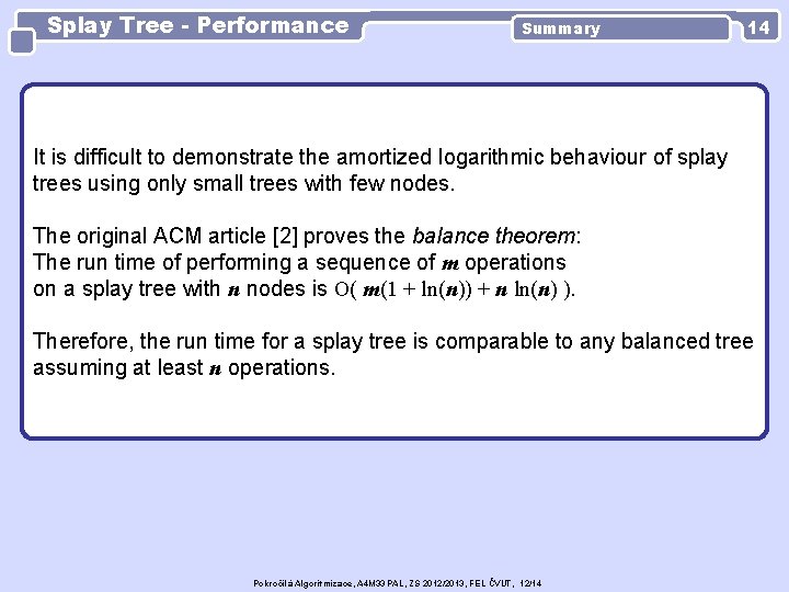
Splay Tree - Performance Summary 14 It is difficult to demonstrate the amortized logarithmic behaviour of splay trees using only small trees with few nodes. The original ACM article [2] proves the balance theorem: The run time of performing a sequence of m operations on a splay tree with n nodes is O( m(1 + ln(n)) + n ln(n) ). Therefore, the run time for a splay tree is comparable to any balanced tree assuming at least n operations. Pokročilá Algoritmizace, A 4 M 33 PAL, ZS 2012/2013, FEL ČVUT, 12/14

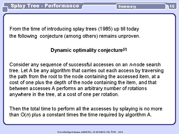
Splay Tree - Performance Summary From the time of introducing splay trees (1985) up till today the following conjecture (among others) remains unproven. Dynamic optimality conjecture[2] Consider any sequence of successful accesses on an n-node search tree. Let A be any algorithm that carries out each access by traversing the path from the root to the node containing the accessed item, at a cost of one plus the depth of the node containing the item, and that between accesses A performs an arbitrary number of rotations anywhere in the tree, at a cost of one per rotation. Then the total time to perform all the accesses by splaying is no more than O(n) plus a constant times the time required by algorithm A. Pokročilá Algoritmizace, A 4 M 33 PAL, ZS 2012/2013, FEL ČVUT, 12/14 15

Splay Tree - Performance Comparisons Advantages: – The amortized run times are similar to that of AVL trees and redblack trees – The implementation is easier – No additional information (height/colour) is required Disadvantages: – The tree will change with read-only operations Pokročilá Algoritmizace, A 4 M 33 PAL, ZS 2012/2013, FEL ČVUT, 12/14 16

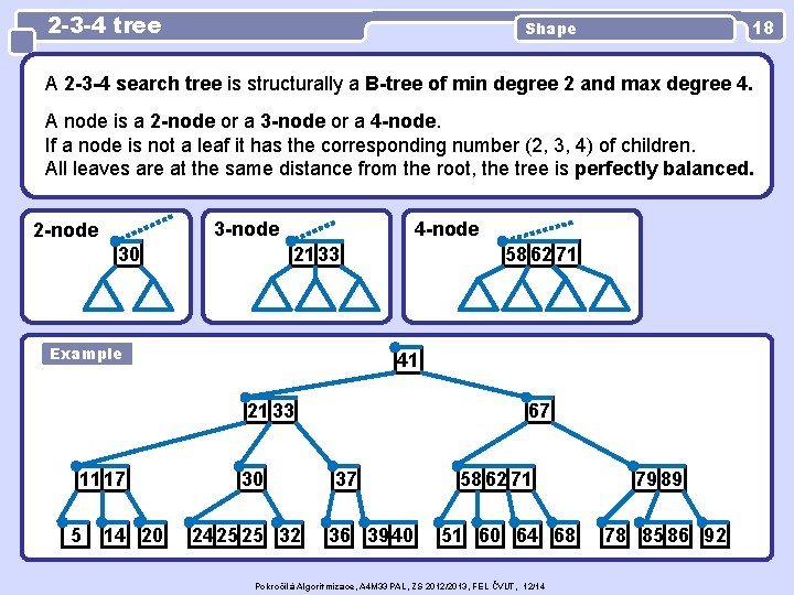
2 -3 -4 tree 18 Shape A 2 -3 -4 search tree is structurally a B-tree of min degree 2 and max degree 4. A node is a 2 -node or a 3 -node or a 4 -node. If a node is not a leaf it has the corresponding number (2, 3, 4) of children. All leaves are at the same distance from the root, the tree is perfectly balanced. 3 -node 2 -node 4 -node 21 33 30 Example 58 62 71 41 21 33 11 17 5 14 20 30 24 25 25 32 67 37 36 39 40 58 62 71 51 60 64 68 Pokročilá Algoritmizace, A 4 M 33 PAL, ZS 2012/2013, FEL ČVUT, 12/14 79 89 78 85 86 92

2 -3 -4 tree Operations Find: As in B-tree Insert: As in B-tree: Find the place for the inserted key x in a leaf and store it there. If necessary, split the leaf and store the median in the parent. Splitting strategy Additional insert rule (like single phase strategy in B-trees): In our way down the tree, whenever we reach a 4 -node (including a leaf), we split it into two 2 -nodes, and move the middle element up to the parent node. This strategy prevents the following from happening: After inserting a key it might be necessary to split all the nodes going from inserted key back to the root. Such outcome is considered to be time consuming. Splitting 4 -nodes on the way down results in sparse occurence of 4 -nodes in the tree, thus the nodes never have to be split recursively bottom-up. Delete: As in B-tree Pokročilá Algoritmizace, A 4 M 33 PAL, ZS 2012/2013, FEL ČVUT, 12/14 19

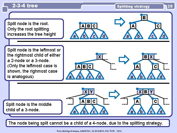
2 -3 -4 tree 20 Splitting strategy B Split node is the root. Only the root splitting increases the tree height A B C a Split node is the leftmost or the rightmost child of either a 2 -node or a 3 -node. (Only the leftmost case is shown, the righmost case is analogous) b A c d a b c X A B C a b A c d a b C b c d X B Y A B C a d B X X Y Split node is the middle child of a 3 -node. C c A d a C b c d The node being split cannot be a child of a 4 -node, due to the splitting strategy. Pokročilá Algoritmizace, A 4 M 33 PAL, ZS 2012/2013, FEL ČVUT, 12/14

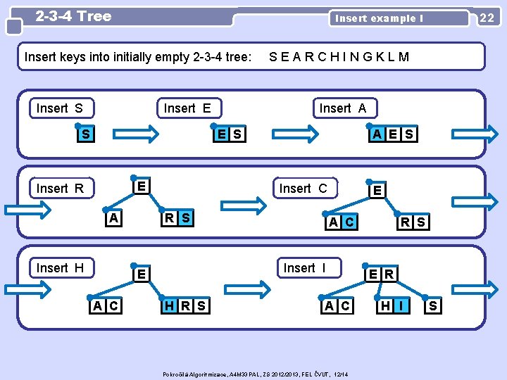
2 -3 -4 Tree Insert keys into initially empty 2 -3 -4 tree: Insert S Insert E S SEARCHINGKLM Insert A E S E Insert R A Insert H A E S Insert C R S E A C Insert I E A C 22 Insert example I H R S A C Pokročilá Algoritmizace, A 4 M 33 PAL, ZS 2012/2013, FEL ČVUT, 12/14 R S E R H I S

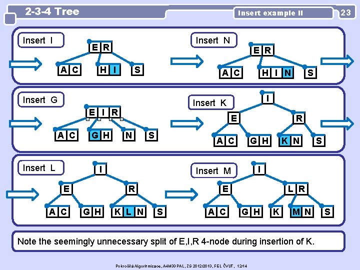
2 -3 -4 Tree Insert I Insert N E R A C H I S Insert L N S A C G H R A C G H K L N K N E S A C S I Insert M R S I E H I N Insert K E I R G H E R A C Insert G A C 23 Insert example II L R G H K M N Note the seemingly unnecessary split of E, I, R 4 -node during insertion of K. Pokročilá Algoritmizace, A 4 M 33 PAL, ZS 2012/2013, FEL ČVUT, 12/14 S

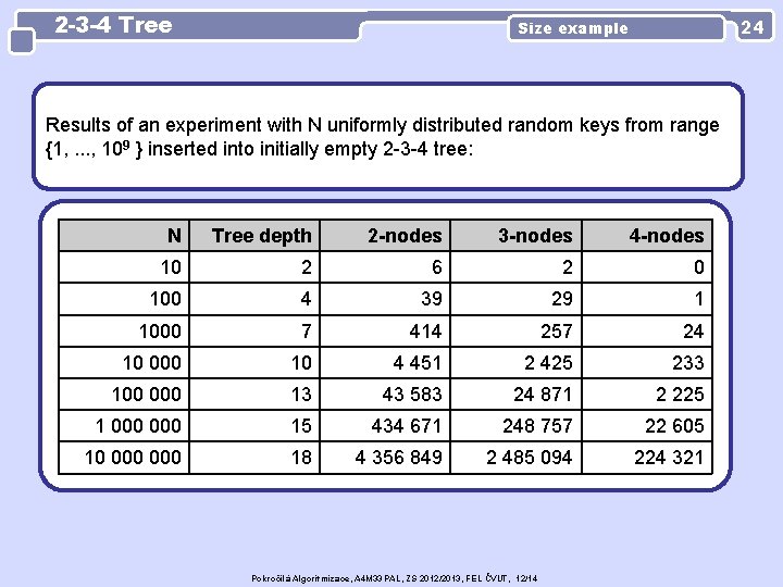
2 -3 -4 Tree 24 Size example Results of an experiment with N uniformly distributed random keys from range {1, . . . , 109 } inserted into initially empty 2 -3 -4 tree: N Tree depth 2 -nodes 3 -nodes 4 -nodes 10 2 6 2 0 100 4 39 29 1 1000 7 414 257 24 10 000 10 4 451 2 425 233 100 000 13 43 583 24 871 2 225 1 000 15 434 671 248 757 22 605 10 000 18 4 356 849 2 485 094 224 321 Pokročilá Algoritmizace, A 4 M 33 PAL, ZS 2012/2013, FEL ČVUT, 12/14

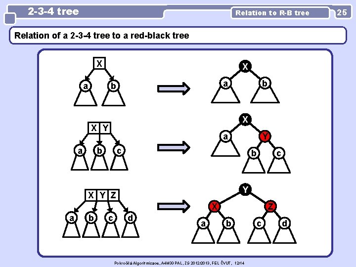
2 -3 -4 tree Relation to R-B tree Relation of a 2 -3 -4 tree to a red-black tree X a b X X Y a b Y c b c Y X Y Z X a b c d a Z b Pokročilá Algoritmizace, A 4 M 33 PAL, ZS 2012/2013, FEL ČVUT, 12/14 c d 25

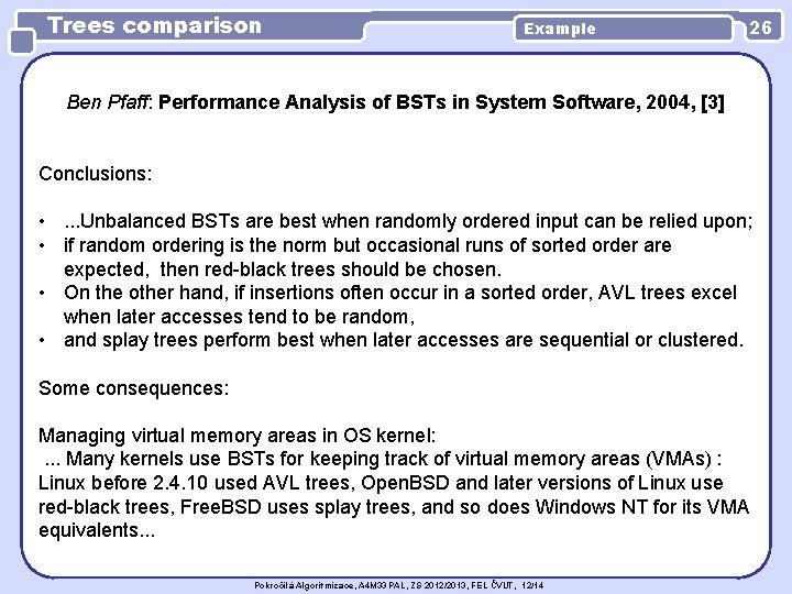
Trees comparison Example 26 Ben Pfaff: Performance Analysis of BSTs in System Software, 2004, [3] Conclusions: • . . . Unbalanced BSTs are best when randomly ordered input can be relied upon; • if random ordering is the norm but occasional runs of sorted order are expected, then red-black trees should be chosen. • On the other hand, if insertions often occur in a sorted order, AVL trees excel when later accesses tend to be random, • and splay trees perform best when later accesses are sequential or clustered. Some consequences: Managing virtual memory areas in OS kernel: . . . Many kernels use BSTs for keeping track of virtual memory areas (VMAs) : Linux before 2. 4. 10 used AVL trees, Open. BSD and later versions of Linux use red-black trees, Free. BSD uses splay trees, and so does Windows NT for its VMA equivalents. . . Pokročilá Algoritmizace, A 4 M 33 PAL, ZS 2012/2013, FEL ČVUT, 12/14

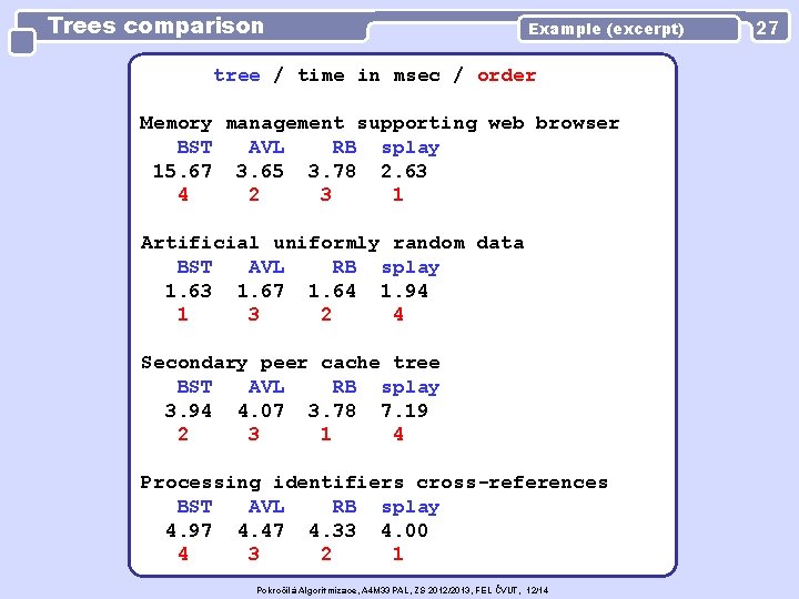
Trees comparison Example (excerpt) tree / time in msec / order Memory management supporting web browser BST AVL RB splay 15. 67 3. 65 3. 78 2. 63 4 2 3 1 Artificial uniformly random data BST AVL RB splay 1. 63 1. 67 1. 64 1. 94 1 3 2 4 Secondary peer cache tree BST AVL RB splay 3. 94 4. 07 3. 78 7. 19 2 3 1 4 Processing identifiers cross-references BST AVL RB splay 4. 97 4. 47 4. 33 4. 00 4 3 2 1 Pokročilá Algoritmizace, A 4 M 33 PAL, ZS 2012/2013, FEL ČVUT, 12/14 27