Spherical Harmonic Lighting The Gritty Details13 Shader Study
 Shader Study 임정환 발표 08/04/15")

 – Realtime Global")
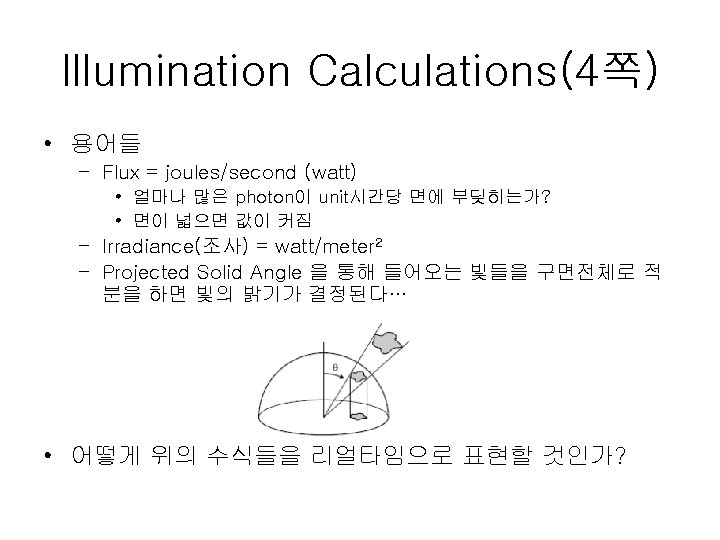
 • Diffuse Surface Reflection • The Rendering Equation, differential angle form")
![• Monte Carlo Integration(7쪽) 지금까지 결과를 코드로 정리해보자. void SH_setup_spherical_samples(SHSample samples[], int sqrt_n_samples)](https://slidetodoc.com/presentation_image/24f5fc40be76ac154c3d42fae7fcd172/image-12.jpg "• Monte Carlo Integration(7쪽) 지금까지 결과를 코드로 정리해보자. void SH_setup_spherical_samples(SHSample samples[], int sqrt_n_samples)")
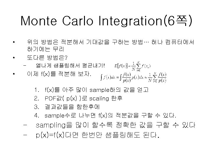
 • Basis function( Bi(x) ) – 어떤 original function을 나타낼수있는 작은")
 • 방금전에 사용된 것은 linear basis functions으로 input function으 로 piecewise")
 • Associated Legendre polynomials – 2개의 아규먼트 l, m은 polynomial을 여러")
 • Associated Legendre polynomials – 각각의 polynomial을 recursive하게 나타낼수있다. – 아래")
 • Associated Legendre polynomials – 소스코드로 한 번 살펴보자")
 • 소스코드를 보자")

- Slides: 20
Spherical Harmonic Lighting: The Gritty Details(1/3) Shader Study 임정환 발표 08/04/15
발표를 하게된 이유 • Shader. X 4 2. 9 Dynamical global illuminations using Tetrahedron environment mapping 모름 • PRT -> 모름 • BRDF -> 모름 • 안에 사용된 SH -> 모름 • OTL • 걍 처음부터…
Introduction • Precomputed Radiance Transfer for Real-Time Rendering. in Dynamic, Slon(02) – Realtime Global Illumination의 한 획을 그은 역사적인 논문 • 문제는? – – 어렵다. 복잡하다. 넘 많은 기초지식을 요해. . OTL • 해서 우리의 Robin Green께서 Spherical Harmonic Lighting: The Gritty Details 이라는 논문을 내셨다!! – 해도 넘 어렵더라 – 공업수학 내용 나오고, 돌아버림
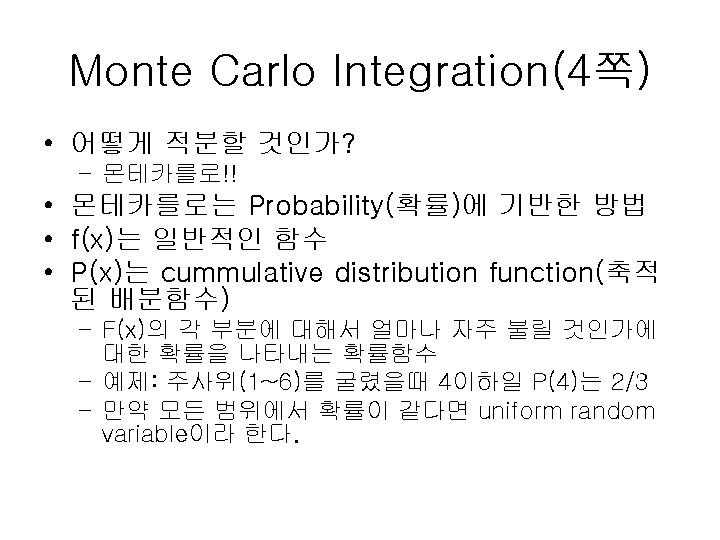
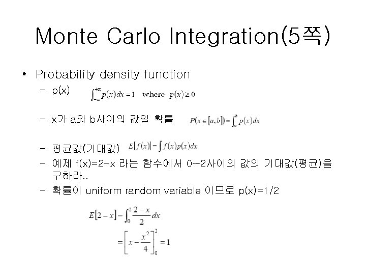
Illumination Calculations(2~3쪽) • Diffuse Surface Reflection • The Rendering Equation, differential angle form
• Monte Carlo Integration(7쪽) 지금까지 결과를 코드로 정리해보자. void SH_setup_spherical_samples(SHSample samples[], int sqrt_n_samples) { // fill an N*N*2 array with uniformly distributed struct SHSample { // samples across the sphere using jittered stratification Vector 3 d sph; int i=0; // array index Vector 3 d vec; double oneover. N = 1. 0/sqrt_n_samples; double *coeff; for(int a=0; a<sqrt_n_samples; a++) { }; for(int b=0; b<sqrt_n_samples; b++) { // generate unbiased distribution of spherical coords double x = (a + random()) * oneover. N; // do not reuse results double y = (b + random()) * oneover. N; // each sample must be random double theta = 2. 0 * acos(sqrt(1. 0 - x)); double phi = 2. 0 * PI * y; samples[i]. sph = Vector 3 d(theta, phi, 1. 0); // convert spherical coords to unit vector Vector 3 d vec(sin(theta)*cos(phi), sin(theta)*sin(phi), cos(theta)); samples[i]. vec = vec; // precompute all SH coefficients for this sample for(int l=0; l<n_bands; ++l) { for(int m=-l; m<=l; ++m) { int index = l*(l+1)+m; samples[i]. coeff[index] = SH(l, m, theta, phi); } } ++i; } } }
Orthogonal Basis Function(8쪽) • Basis function( Bi(x) ) – 어떤 original function을 나타낼수있는 작은 조각 – basis function을 scaling, sum을 통해 original function을 근사 화할 수 있다. (이러한 과정을 projection한다고 한다) 옆에 과정을 통해 coefficient를 구 할 수 있다. 구해진 coefficient와 basis를 한 번 더 곱한 후 그 결과값을 sum하자
Orthogonal Basis Function(9쪽) • 방금전에 사용된 것은 linear basis functions으로 input function으 로 piecewise linear approximation(구분적 선형 근사)을 준다. • 여러 basis function이 있지만 orthogonal polynomials라 불리는 것 이 많이 사용됨 • Orthogonal polynomials(직교 다항식) – 성질 – 직관적으로 다항식들간의 간섭하지 않는다는 것을 알 수 있다. – 가장 유명한 것 중 Legendre polynomials 라 불리는 것이 있다. – Associated Legendre polynomials • symbol로 P라고 표현 • l과 m으로 표현 (-1~1사이) • real number(실수)를 반환
Orthogonal Basis Function(9쪽) • Associated Legendre polynomials – 2개의 아규먼트 l, m은 polynomial을 여러 개의 function band로 나눈다. – l은 band index , 0을 포함한 양수 The first six associated – m은 0~l 사이의 값 Legendre polynomials. 위와 같이 n개면 n(n+1)개의 coefficient를 구한다.
Orthogonal Basis Function(10쪽) • Associated Legendre polynomials – 각각의 polynomial을 recursive하게 나타낼수있다. – 아래 세가지 법칙에 따라. .
Orthogonal Basis Function(10~11 쪽) • Associated Legendre polynomials – 소스코드로 한 번 살펴보자
Spherical Harmonics(13쪽) • 소스코드를 보자
Spherical Harmonics