Speech Processing Speech Recognition August 12 2005 6112021

Speech Processing Speech Recognition August 12, 2005 6/11/2021 1

Speech Recognition l Applications of Speech Recognition (ASR) ¡ ¡ ¡ ¡ 6/11/2021 Dictation Telephone-based Information (directions, air travel, banking, etc) Hands-free (in car) Speaker Identification Language Identification Second language ('L 2') (accent reduction) Audio archive searching 2

LVCSR Large Vocabulary Continuous Speech Recognition l ~20, 000 -64, 000 words l Speaker independent (vs. speaker-dependent) l Continuous speech (vs isolated-word) l 6/11/2021 3

LVCSR Design Intuition Build a statistical model of the speech-to-words process • Collect lots and lots of speech, and transcribe all the words. • Train the model on the labeled speech • Paradigm: Supervised Machine Learning + Search • 6/11/2021 4

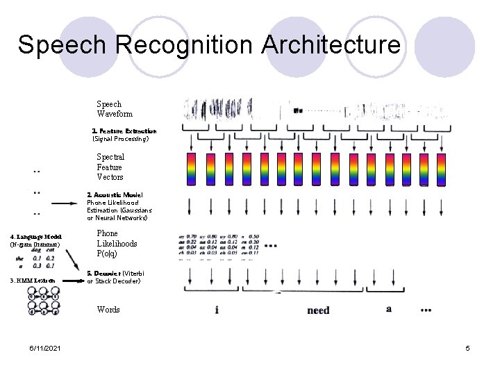
Speech Recognition Architecture Speech Waveform 1. Feature Extraction (Signal Processing) Spectral Feature Vectors 2. Acoustic Model Phone Likelihood Estimation (Gaussians or Neural Networks) 4. Language Model (N-gram Grammar) 3. HMM Lexicon Phone Likelihoods P(o|q) 5. Decoder (Viterbi or Stack Decoder) Words 6/11/2021 5

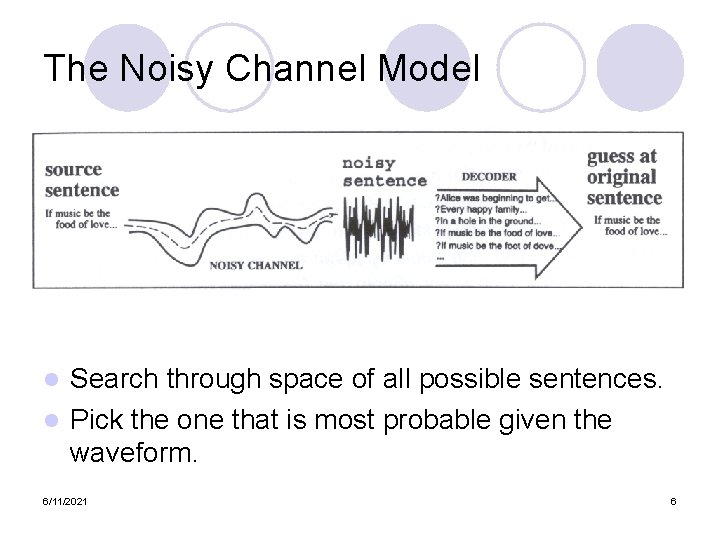
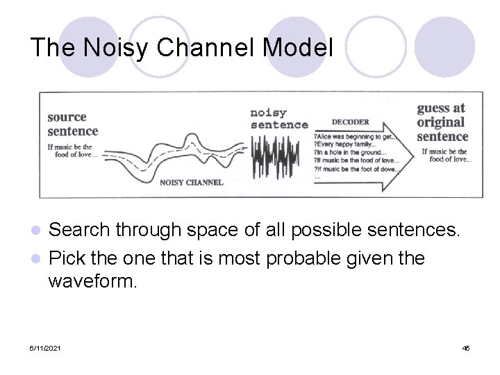
The Noisy Channel Model Search through space of all possible sentences. l Pick the one that is most probable given the waveform. l 6/11/2021 6

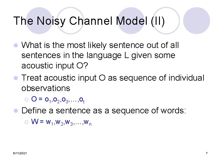
The Noisy Channel Model (II) What is the most likely sentence out of all sentences in the language L given some acoustic input O? l Treat acoustic input O as sequence of individual observations l ¡ l O = o 1, o 2, o 3, …, ot Define a sentence as a sequence of words: ¡ 6/11/2021 W = w 1, w 2, w 3, …, wn 7

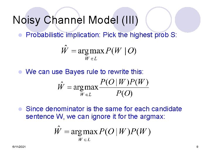
Noisy Channel Model (III) l Probabilistic implication: Pick the highest prob S: l We can use Bayes rule to rewrite this: l Since denominator is the same for each candidate sentence W, we can ignore it for the argmax: 6/11/2021 8

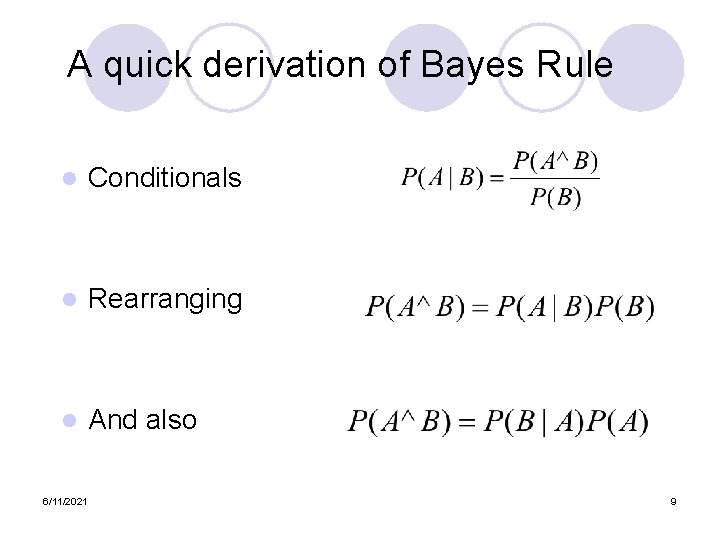
A quick derivation of Bayes Rule l Conditionals l Rearranging l And also 6/11/2021 9

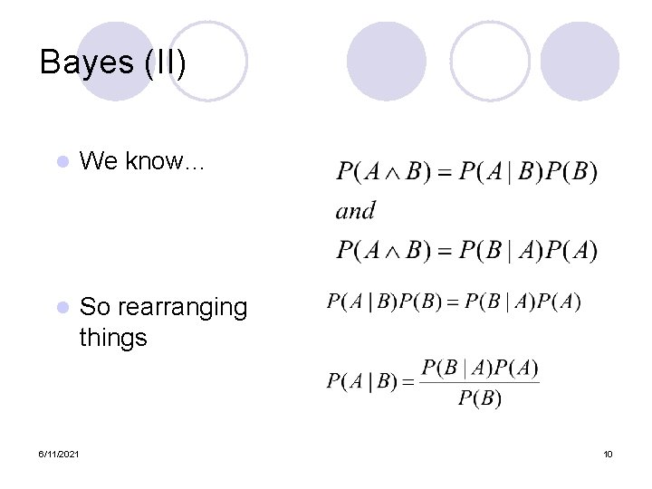
Bayes (II) l We know… l So rearranging things 6/11/2021 10

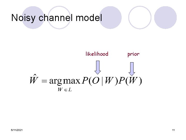
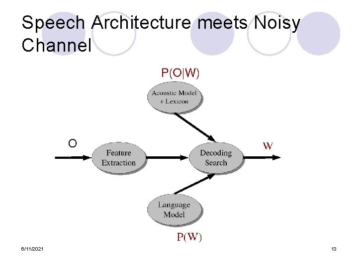
Noisy channel model likelihood 6/11/2021 prior 11

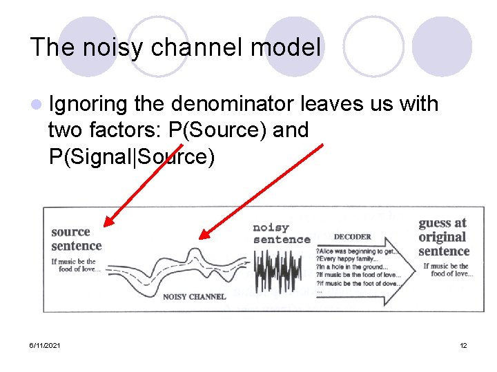
The noisy channel model l Ignoring the denominator leaves us with two factors: P(Source) and P(Signal|Source) 6/11/2021 12

Speech Architecture meets Noisy Channel 6/11/2021 13

Five easy pieces l l l Feature extraction Acoustic Modeling HMMs, Lexicons, and Pronunciation Decoding Language Modeling 6/11/2021 14

Feature Extraction l Digitize Speech l Extract Frames 6/11/2021 15

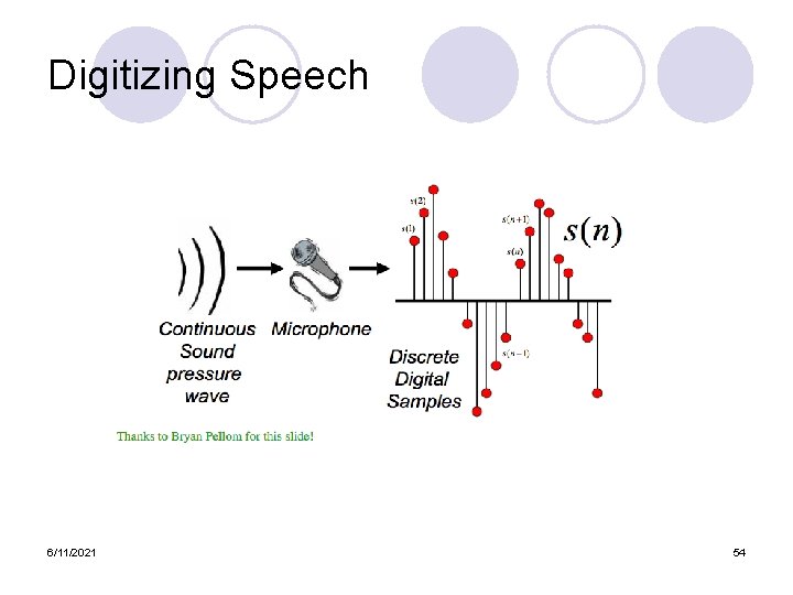
Digitizing Speech 6/11/2021 16

Digitizing Speech (A-D) l Sampling: ¡ measuring amplitude of signal at time t ¡ 16, 000 Hz (samples/sec) Microphone (“Wideband”): ¡ 8, 000 Hz (samples/sec) Telephone ¡ Why? Need at least 2 samples per cycle l max measurable frequency is half sampling rate l Human speech < 10, 000 Hz, so need max 20 K l Telephone filtered at 4 K, so 8 K is enough l 6/11/2021 17

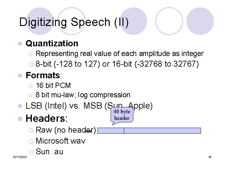
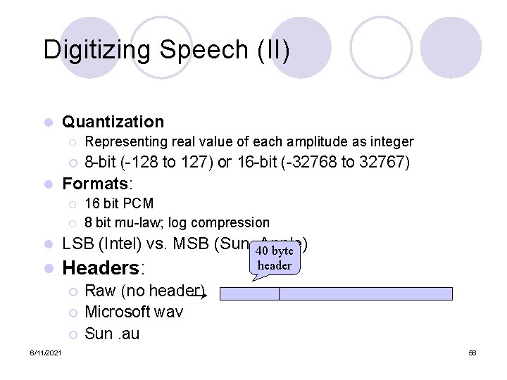
Digitizing Speech (II) l l Quantization ¡ Representing real value of each amplitude as integer ¡ 8 -bit (-128 to 127) or 16 -bit (-32768 to 32767) Formats: ¡ ¡ l 16 bit PCM 8 bit mu-law; log compression LSB (Intel) vs. MSB (Sun, Apple) l Headers: ¡ Raw (no header) ¡ Microsoft wav ¡ Sun. au 6/11/2021 40 byte header 18

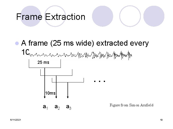
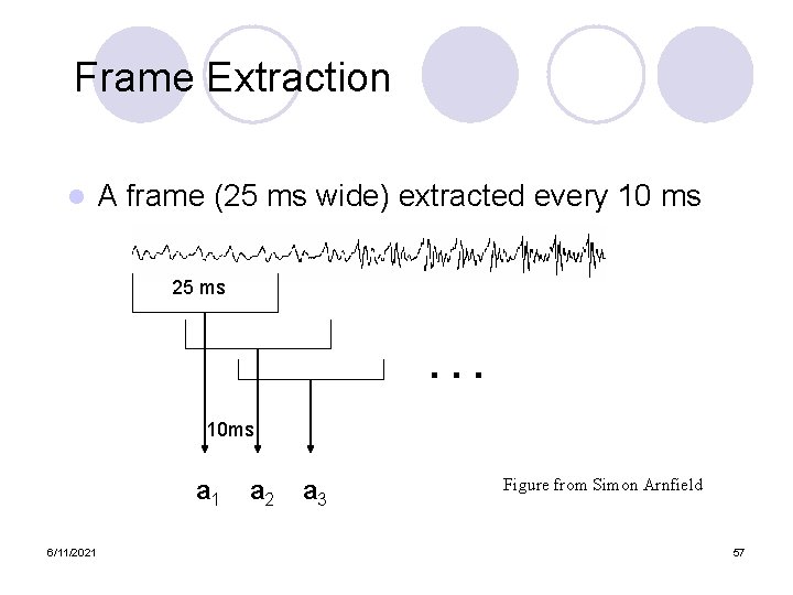
Frame Extraction l. A frame (25 ms wide) extracted every 10 ms 25 ms . . . 10 ms a 1 6/11/2021 a 2 a 3 Figure from Simon Arnfield 19

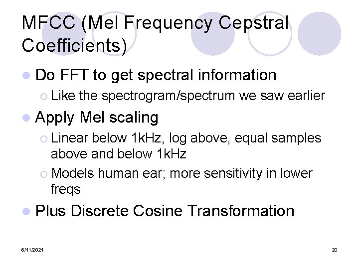
MFCC (Mel Frequency Cepstral Coefficients) l Do FFT to get spectral information ¡ Like l Apply the spectrogram/spectrum we saw earlier Mel scaling ¡ Linear below 1 k. Hz, log above, equal samples above and below 1 k. Hz ¡ Models human ear; more sensitivity in lower freqs l Plus 6/11/2021 Discrete Cosine Transformation 20

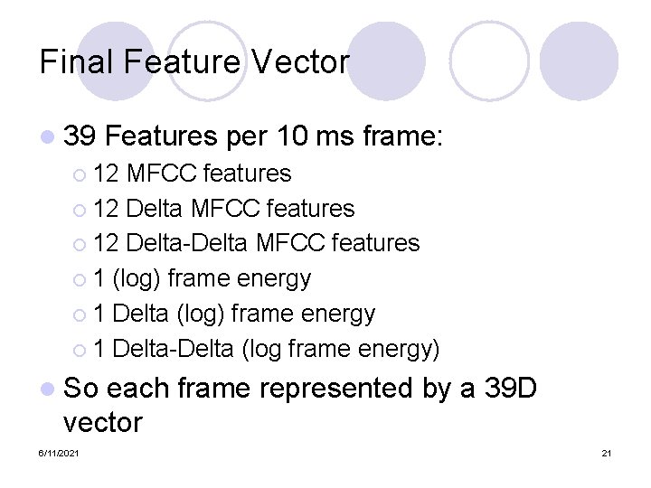
Final Feature Vector l 39 Features per 10 ms frame: ¡ 12 MFCC features ¡ 12 Delta-Delta MFCC features ¡ 1 (log) frame energy ¡ 1 Delta-Delta (log frame energy) l So each frame represented by a 39 D vector 6/11/2021 21

Where we are Given: a sequence of acoustic feature vectors, one every 10 ms l Goal: output a string of words l We’ll spend 6 lectures on how to do this l Rest of today: l ¡ ¡ Markov Models Hidden Markov Models in the abstract l l ¡ 6/11/2021 Forward Algorithm Viterbi Algorithm Start of HMMs for speech 22

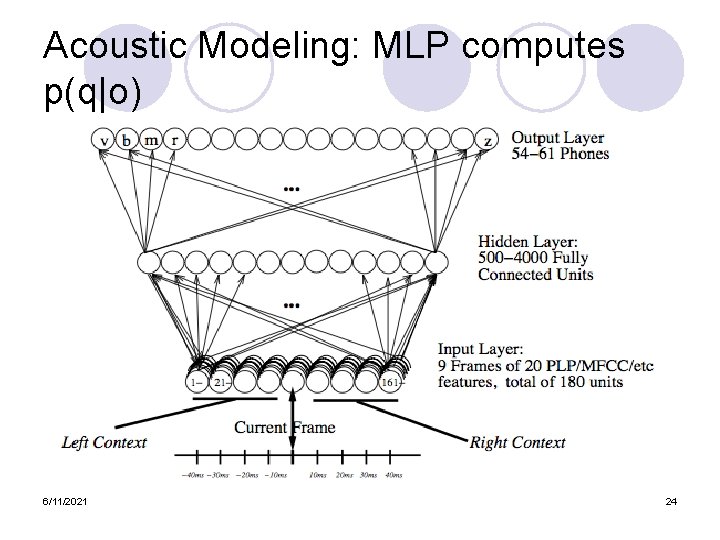
Acoustic Modeling Given a 39 d vector corresponding to the observation of one frame oi l And given a phone q we want to detect l Compute p(oi|q) l Most popular method: l ¡ l GMM (Gaussian mixture models) Other methods ¡ 6/11/2021 MLP (multi-layer perceptron) 23

Acoustic Modeling: MLP computes p(q|o) 6/11/2021 24

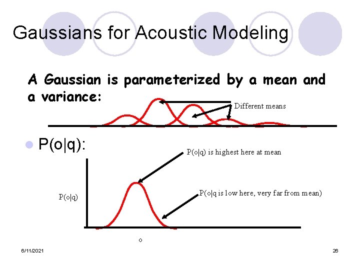
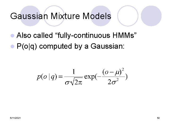
Gaussian Mixture Models l Also called “fully-continuous HMMs” l P(o|q) computed by a Gaussian: 6/11/2021 25

Gaussians for Acoustic Modeling A Gaussian is parameterized by a mean and a variance: Different means l P(o|q): P(o|q) is highest here at mean P(o|q is low here, very far from mean) P(o|q) o 6/11/2021 26

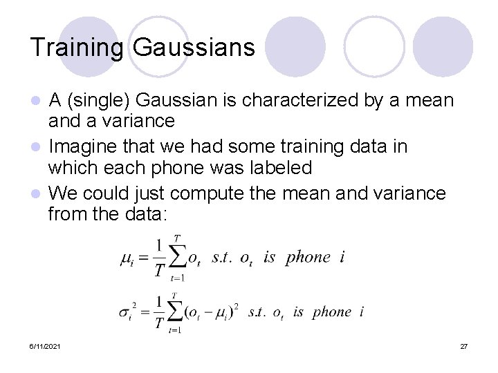
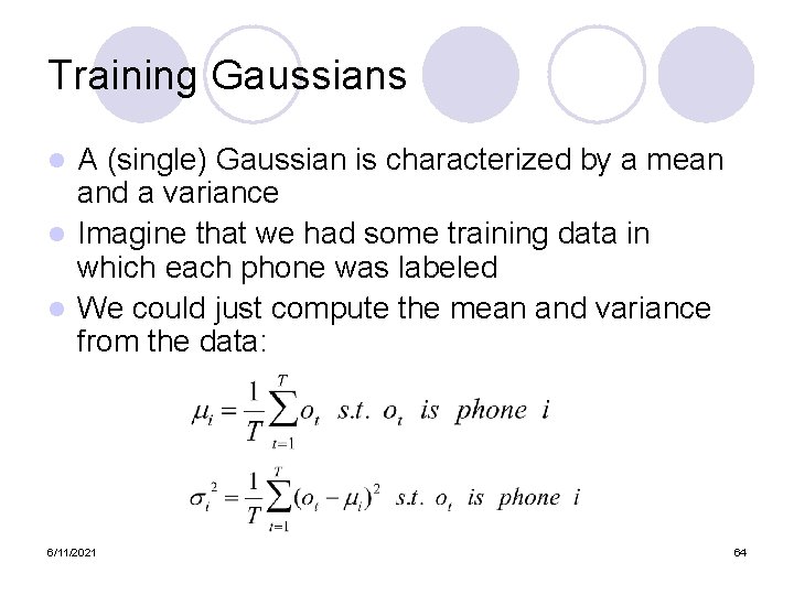
Training Gaussians A (single) Gaussian is characterized by a mean and a variance l Imagine that we had some training data in which each phone was labeled l We could just compute the mean and variance from the data: l 6/11/2021 27

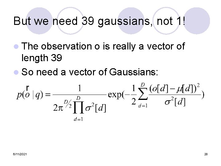
But we need 39 gaussians, not 1! l The observation o is really a vector of length 39 l So need a vector of Gaussians: 6/11/2021 28

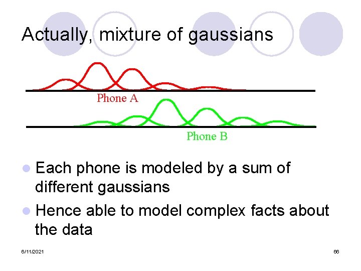
Actually, mixture of gaussians Phone A Phone B l Each phone is modeled by a sum of different gaussians l Hence able to model complex facts about the data 6/11/2021 29

Gaussians acoustic modeling l Summary: each phone is represented by a GMM parameterized by ¡M mixture weights ¡ M mean vectors ¡ M covariance matrices Usually assume covariance matrix is diagonal l I. e. just keep separate variance for each cepstral feature l 6/11/2021 30

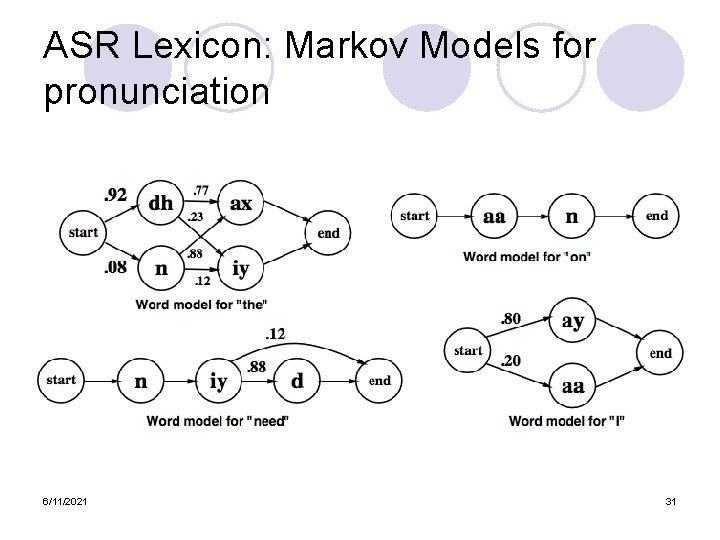
ASR Lexicon: Markov Models for pronunciation 6/11/2021 31

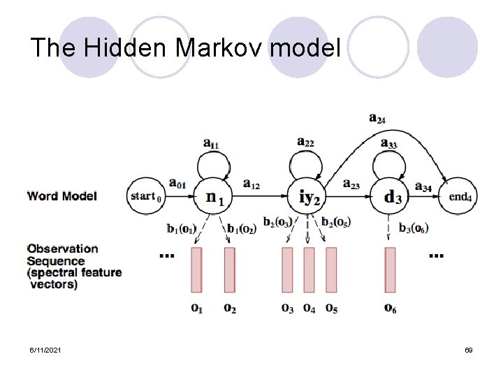
The Hidden Markov model 6/11/2021 32

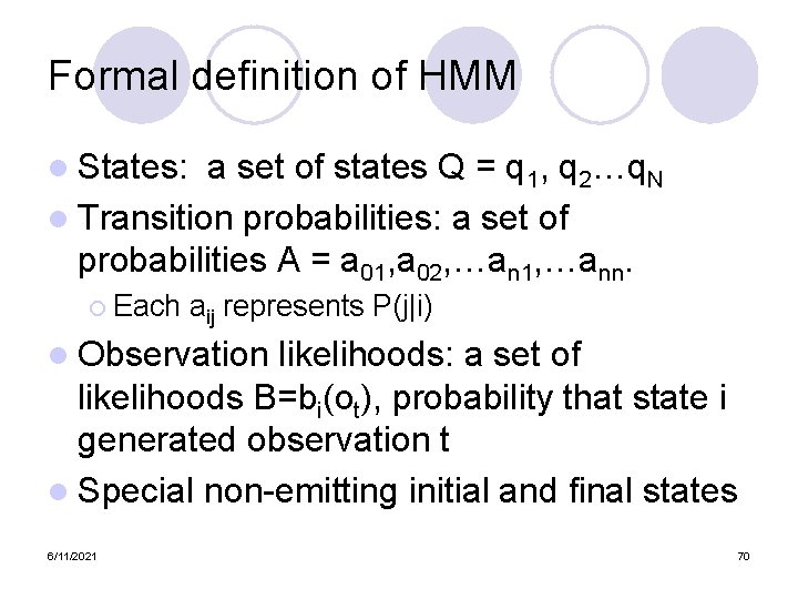
Formal definition of HMM l States: a set of states Q = q 1, q 2…q. N l Transition probabilities: a set of probabilities A = a 01, a 02, …an 1, …ann. ¡ Each aij represents P(j|i) l Observation likelihoods: a set of likelihoods B=bi(ot), probability that state i generated observation t l Special non-emitting initial and final states 6/11/2021 33

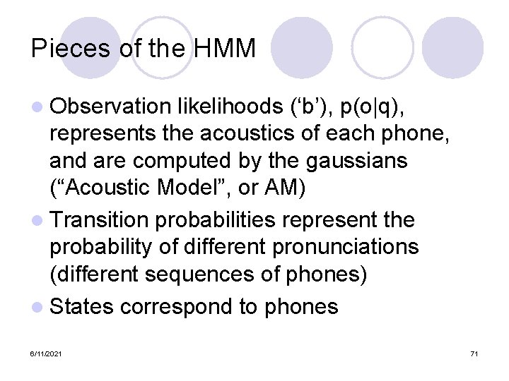
Pieces of the HMM l Observation likelihoods (‘b’), p(o|q), represents the acoustics of each phone, and are computed by the gaussians (“Acoustic Model”, or AM) l Transition probabilities represent the probability of different pronunciations (different sequences of phones) l States correspond to phones 6/11/2021 34

Pieces of the HMM l Actually, I lied when I say states correspond to phones l Actually states usually correspond to triphones l CHEESE (phones): ch iy z l CHEESE (triphones) #-ch+iy, ch-iy+z, iyz+# 6/11/2021 35

Pieces of the HMM l Actually, I lied again when I said states correspond to triphones l In fact, each triphone has 3 states for beginning, middle, and end of the triphone. l 6/11/2021 36

A real HMM 6/11/2021 37

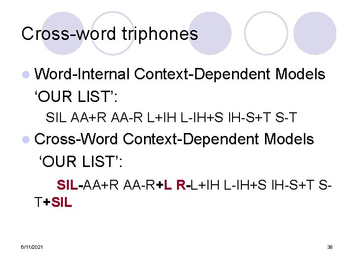
Cross-word triphones l Word-Internal Context-Dependent Models ‘OUR LIST’: SIL AA+R AA-R L+IH L-IH+S IH-S+T S-T l Cross-Word Context-Dependent Models ‘OUR LIST’: SIL-AA+R AA-R+L R-L+IH L-IH+S IH-S+T ST+SIL 6/11/2021 38

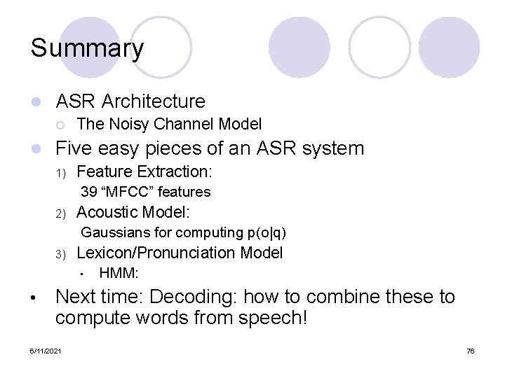
Summary l ASR Architecture ¡ l The Noisy Channel Model Five easy pieces of an ASR system 1) Feature Extraction: 39 “MFCC” features 2) Acoustic Model: Gaussians for computing p(o|q) 3) Lexicon/Pronunciation Model • • HMM: Next time: Decoding: how to combine these to compute words from speech! 6/11/2021 39

Perceptual properties l Pitch: perceptual correlate of frequency l Loudness: perceptual correlate of power, which is related to square of amplitude 6/11/2021 40

Speech Recognition l Applications of Speech Recognition (ASR) ¡ Dictation ¡ Telephone-based Information (directions, air travel, banking, etc) ¡ Hands-free (in car) ¡ Speaker Identification ¡ Language Identification ¡ Second language ('L 2') (accent reduction) ¡ Audio archive searching 6/11/2021 41

LVCSR l Large Vocabulary Continuous Speech Recognition l ~20, 000 -64, 000 words l Speaker independent (vs. speakerdependent) l Continuous speech (vs isolated-word) 6/11/2021 42

LVCSR Design Intuition Build a statistical model of the speech-towords process • Collect lots and lots of speech, and transcribe all the words. • Train the model on the labeled speech • Paradigm: Supervised Machine Learning + Search • 6/11/2021 43

Speech Recognition Architecture Speech Waveform 1. Feature Extraction (Signal Processing) Spectral Feature Vectors 2. Acoustic Model Phone Likelihood Estimation (Gaussians or Neural Networks) 4. Language Model (N-gram Grammar) 3. HMM Lexicon Phone Likelihoods P(o|q) 5. Decoder (Viterbi or Stack Decoder) Words 6/11/2021 44

The Noisy Channel Model Search through space of all possible sentences. l Pick the one that is most probable given the waveform. l 6/11/2021 45

The Noisy Channel Model (II) What is the most likely sentence out of all sentences in the language L given some acoustic input O? l Treat acoustic input O as sequence of individual observations l ¡ l O = o 1, o 2, o 3, …, ot Define a sentence as a sequence of words: ¡ 6/11/2021 W = w 1, w 2, w 3, …, wn 46

Noisy Channel Model (III) l Probabilistic implication: Pick the highest prob S: l We can use Bayes rule to rewrite this: l Since denominator is the same for each candidate sentence W, we can ignore it for the argmax: 6/11/2021 47

A quick derivation of Bayes Rule l Conditionals l Rearranging l And also 6/11/2021 48

Bayes (II) l We know… l So rearranging things 6/11/2021 49

Noisy channel model likelihood 6/11/2021 prior 50

The noisy channel model l Ignoring the denominator leaves us with two factors: P(Source) and P(Signal|Source) 6/11/2021 51

Five easy pieces l Feature extraction l Acoustic Modeling l HMMs, Lexicons, and Pronunciation l Decoding l Language Modeling 6/11/2021 52

Feature Extraction l Digitize Speech l Extract Frames 6/11/2021 53

Digitizing Speech 6/11/2021 54

Digitizing Speech (A-D) l Sampling: ¡ ¡ measuring amplitude of signal at time t 16, 000 Hz (samples/sec) Microphone (“Wideband”): 8, 000 Hz (samples/sec) Telephone Why? l l 6/11/2021 Need at least 2 samples per cycle max measurable frequency is half sampling rate Human speech < 10, 000 Hz, so need max 20 K Telephone filtered at 4 K, so 8 K is enough 55

Digitizing Speech (II) l Quantization ¡ Representing real value of each amplitude as integer 8 -bit (-128 to 127) or 16 -bit (-32768 to 32767) l Formats: ¡ ¡ ¡ l l LSB (Intel) vs. MSB (Sun, 40 Apple) byte Headers: ¡ ¡ ¡ 6/11/2021 16 bit PCM 8 bit mu-law; log compression header Raw (no header) Microsoft wav Sun. au 56

Frame Extraction l A frame (25 ms wide) extracted every 10 ms 25 ms . . . 10 ms a 1 6/11/2021 a 2 a 3 Figure from Simon Arnfield 57

MFCC (Mel Frequency Cepstral Coefficients) l Do FFT to get spectral information ¡ Like l Apply the spectrogram/spectrum we saw earlier Mel scaling ¡ Linear below 1 k. Hz, log above, equal samples above and below 1 k. Hz ¡ Models human ear; more sensitivity in lower freqs l Plus 6/11/2021 Discrete Cosine Transformation 58

Final Feature Vector l 39 Features per 10 ms frame: ¡ 12 MFCC features ¡ 12 Delta-Delta MFCC features ¡ 1 (log) frame energy ¡ 1 Delta-Delta (log frame energy) l So each frame represented by a 39 D vector 6/11/2021 59

Acoustic Modeling Given a 39 d vector corresponding to the observation of one frame oi l And given a phone q we want to detect l Compute p(oi|q) l Most popular method: l ¡ l GMM (Gaussian mixture models) Other methods ¡ 6/11/2021 MLP (multi-layer perceptron) 60

Acoustic Modeling: MLP computes p(q|o) 6/11/2021 61

Gaussian Mixture Models l Also called “fully-continuous HMMs” l P(o|q) computed by a Gaussian: 6/11/2021 62

Gaussians for Acoustic Modeling A Gaussian is parameterized by a mean and a variance: Different means l P(o|q): P(o|q) is highest here at mean P(o|q is low here, very far from mean) P(o|q) o 6/11/2021 63

Training Gaussians A (single) Gaussian is characterized by a mean and a variance l Imagine that we had some training data in which each phone was labeled l We could just compute the mean and variance from the data: l 6/11/2021 64

But we need 39 gaussians, not 1! l The observation o is really a vector of length 39 l So need a vector of Gaussians: 6/11/2021 65

Actually, mixture of gaussians Phone A Phone B l Each phone is modeled by a sum of different gaussians l Hence able to model complex facts about the data 6/11/2021 66

Gaussians acoustic modeling l Summary: each phone is represented by a GMM parameterized by ¡M mixture weights ¡ M mean vectors ¡ M covariance matrices Usually assume covariance matrix is diagonal l I. e. just keep separate variance for each cepstral feature l 6/11/2021 67

ASR Lexicon: Markov Models for pronunciation 6/11/2021 68

The Hidden Markov model 6/11/2021 69

Formal definition of HMM l States: a set of states Q = q 1, q 2…q. N l Transition probabilities: a set of probabilities A = a 01, a 02, …an 1, …ann. ¡ Each aij represents P(j|i) l Observation likelihoods: a set of likelihoods B=bi(ot), probability that state i generated observation t l Special non-emitting initial and final states 6/11/2021 70

Pieces of the HMM l Observation likelihoods (‘b’), p(o|q), represents the acoustics of each phone, and are computed by the gaussians (“Acoustic Model”, or AM) l Transition probabilities represent the probability of different pronunciations (different sequences of phones) l States correspond to phones 6/11/2021 71

Pieces of the HMM l Actually, I lied when I say states correspond to phones l Actually states usually correspond to triphones l CHEESE (phones): ch iy z l CHEESE (triphones) #-ch+iy, ch-iy+z, iyz+# 6/11/2021 72

Pieces of the HMM l Actually, I lied again when I said states correspond to triphones l In fact, each triphone has 3 states for beginning, middle, and end of the triphone. l 6/11/2021 73

A real HMM 6/11/2021 74

Cross-word triphones l Word-Internal Context-Dependent Models ‘OUR LIST’: SIL AA+R AA-R L+IH L-IH+S IH-S+T S-T l Cross-Word Context-Dependent Models ‘OUR LIST’: SIL-AA+R AA-R+L R-L+IH L-IH+S IH-S+T ST+SIL 6/11/2021 75

Summary l ASR Architecture ¡ l The Noisy Channel Model Five easy pieces of an ASR system 1) Feature Extraction: 39 “MFCC” features 2) Acoustic Model: Gaussians for computing p(o|q) 3) Lexicon/Pronunciation Model • • HMM: Next time: Decoding: how to combine these to compute words from speech! 6/11/2021 76