Speech Processing Speaker Recognition Speaker Recognition u Definitions

Speech Processing Speaker Recognition

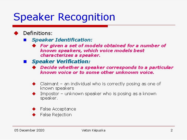
Speaker Recognition u Definitions: n Speaker Identification: u For given a set of models obtained for a number of known speakers, which voice models best characterizes a speaker. n Speaker Verification: u Decide whether a speaker corresponds to a particular known voice or to some other unknown voice. u Claimant – an individual who is correctly posing as one of known speakers u Impostor – unknown speaker who is posing as a known speaker. u False Acceptance u False Rejection 05 December 2020 Veton Këpuska 2

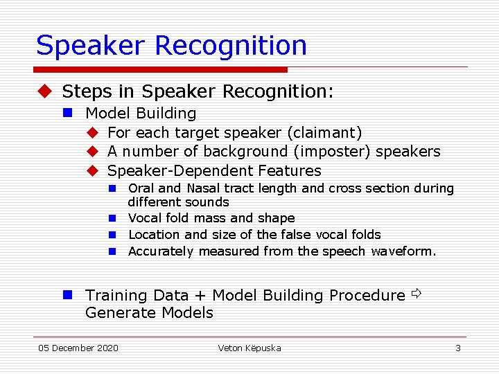
Speaker Recognition u Steps in Speaker Recognition: n Model Building u For each target speaker (claimant) u A number of background (imposter) speakers u Speaker-Dependent Features n Oral and Nasal tract length and cross section during different sounds n Vocal fold mass and shape n Location and size of the false vocal folds n Accurately measured from the speech waveform. n Training Data + Model Building Procedure Generate Models 05 December 2020 Veton Këpuska ⇨ 3

Speaker Recognition u In practice difficult to derive speech anatomy features from the speech waveform. u Use conventional methods to extract features: n Constant-Q filter bank n Spectral Based Features 05 December 2020 Veton Këpuska 4

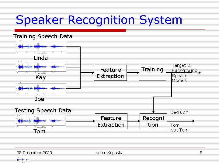
Speaker Recognition System Training Speech Data Linda Kay Feature Extraction Training Target & Background Speaker Models Joe Testing Speech Data Feature Extraction Tom 05 December 2020 Veton Këpuska Recogni tion Decision: Tom Not Tom 5

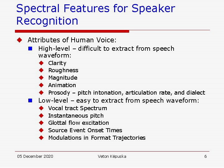
Spectral Features for Speaker Recognition u Attributes of Human Voice: n High-level – difficult to extract from speech waveform: u u u Clarity Roughness Magnitude Animation Prosody – pitch intonation, articulation rate, and dialect n Low-level – easy to extract from speech waveform: u u u Vocal tract Spectrum Instantaneous pitch Glottal flow excitation Source Event Onset Times Modulations in Format Trajectories 05 December 2020 Veton Këpuska 6

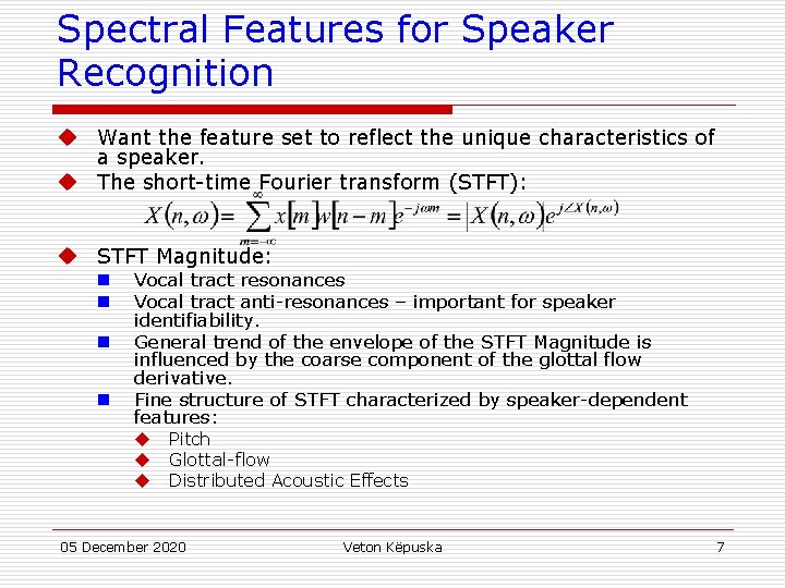
Spectral Features for Speaker Recognition u Want the feature set to reflect the unique characteristics of a speaker. u The short-time Fourier transform (STFT): u STFT Magnitude: n n Vocal tract resonances Vocal tract anti-resonances – important for speaker identifiability. General trend of the envelope of the STFT Magnitude is influenced by the coarse component of the glottal flow derivative. Fine structure of STFT characterized by speaker-dependent features: u Pitch u Glottal-flow u Distributed Acoustic Effects 05 December 2020 Veton Këpuska 7

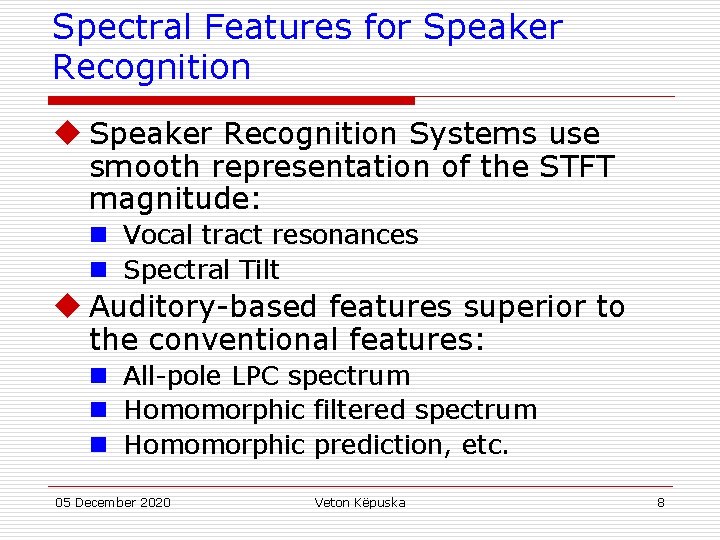
Spectral Features for Speaker Recognition u Speaker Recognition Systems use smooth representation of the STFT magnitude: n Vocal tract resonances n Spectral Tilt u Auditory-based features superior to the conventional features: n All-pole LPC spectrum n Homomorphic filtered spectrum n Homomorphic prediction, etc. 05 December 2020 Veton Këpuska 8

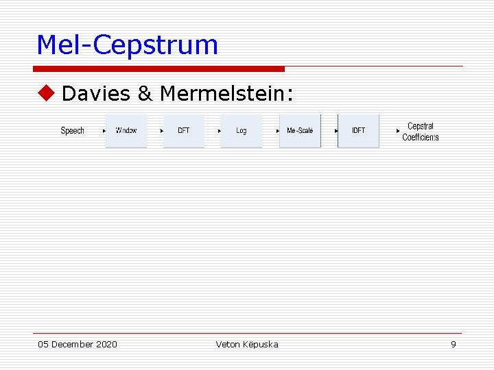
Mel-Cepstrum u Davies & Mermelstein: 05 December 2020 Veton Këpuska 9

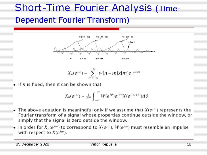
Short-Time Fourier Analysis (Time- Dependent Fourier Transform) 05 December 2020 Veton Këpuska 10

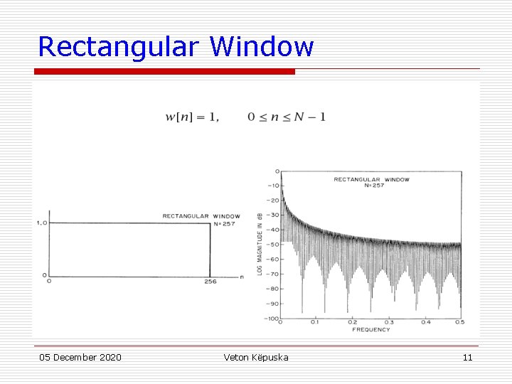
Rectangular Window 05 December 2020 Veton Këpuska 11

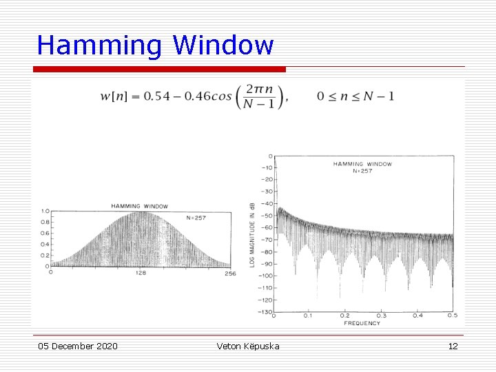
Hamming Window 05 December 2020 Veton Këpuska 12

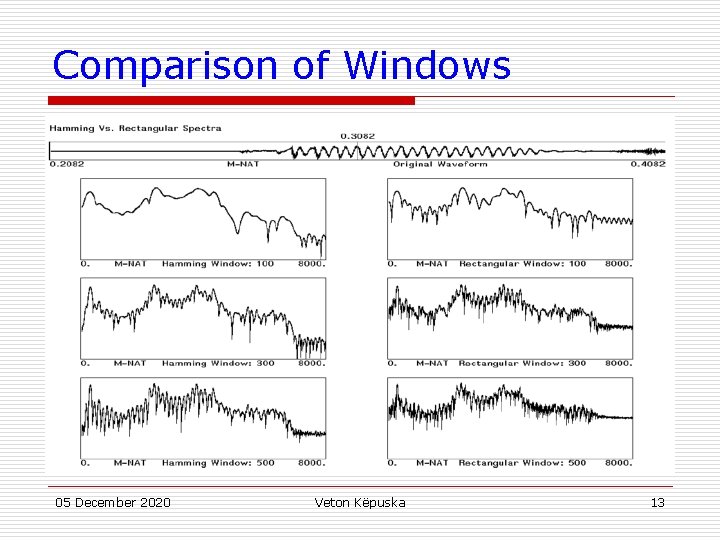
Comparison of Windows 05 December 2020 Veton Këpuska 13

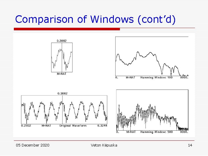
Comparison of Windows (cont’d) 05 December 2020 Veton Këpuska 14

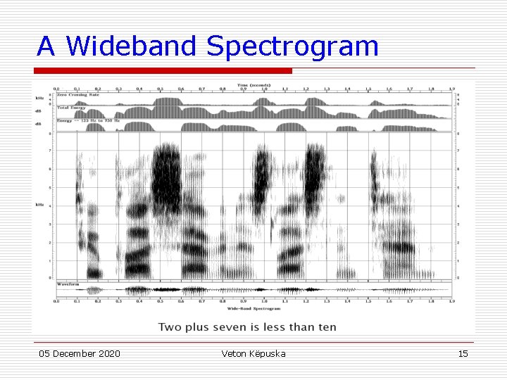
A Wideband Spectrogram 05 December 2020 Veton Këpuska 15

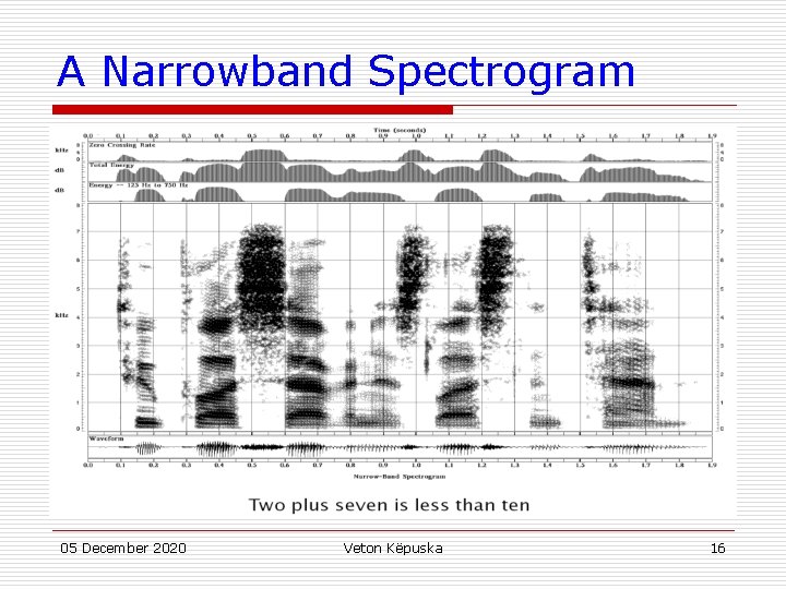
A Narrowband Spectrogram 05 December 2020 Veton Këpuska 16

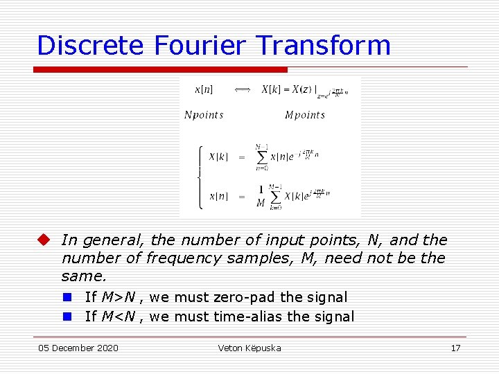
Discrete Fourier Transform u In general, the number of input points, N, and the number of frequency samples, M, need not be the same. n If M>N , we must zero-pad the signal n If M<N , we must time-alias the signal 05 December 2020 Veton Këpuska 17

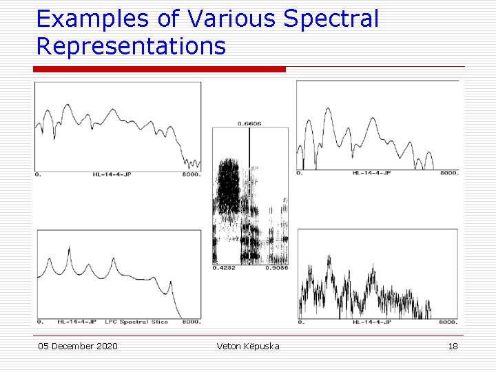
Examples of Various Spectral Representations 05 December 2020 Veton Këpuska 18

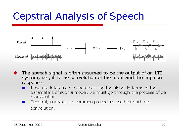
Cepstral Analysis of Speech u The speech signal is often assumed to be the output of an LTI system; i. e. , it is the convolution of the input and the impulse response. n n If we are interested in characterizing the signal in terms of the parameters of such a model, we must go through the process of de -convolution. Cepstral, analysis is a common procedure used for such deconvolution. 05 December 2020 Veton Këpuska 19

Cepstral Analysis u Cepstral analysis for convolution is based on the observation that: x[n]= x 1[n] * x 2[n] ⇒ X (z)= X 1(z)X 2(z) By taking the complex logarithm of X(z), then log{X (z)} =log{X 1(z)} + log{X 2(z)} = u If the complex logarithm is unique, and if then is a valid z-transform, The two convolved signals will be additive in this new, cepstral domain. u If we restrict ourselves to the unit circle, z = ej , then: u It can be shown that one approach to dealing with the problem of uniqueness is to require that arg{X(ejω)} be a continuous, odd, periodic function of ω. 05 December 2020 Veton Këpuska 20

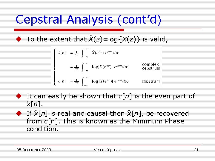
Cepstral Analysis (cont’d) ^ u To the extent that X(z)=log{X(z)} is valid, u It can easily be shown that c[n] is the even part of ^ x[n]. ^ ^ u If x[n] is real and causal then x[n], be recovered from c[n]. This is known as the Minimum Phase condition. 05 December 2020 Veton Këpuska 21

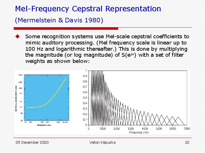
Mel-Frequency Cepstral Representation (Mermelstein & Davis 1980) u Some recognition systems use Mel-scale cepstral coefficients to mimic auditory processing. (Mel frequency scale is linear up to 100 Hz and logarithmic thereafter. ) This is done by multiplying the magnitude (or log magnitude) of S(ej ) with a set of filter weights as shown below: 05 December 2020 Veton Këpuska 22

References 1. Tohkura, Y. , “A Weighted Cepstral Distance Measure for Speech Recognition, " IEEE Trans. ASSP, Vol. ASSP -35, No. 10, 1414 -1422, 1987. 2. Mermelstein, P. and Davis, S. , “Comparison of Parametric Representations for Monosyllabic Word Recognition in Continuously Spoken Sentences, " IEEE Trans. ASSP, Vol. ASSP-28, No. 4, 357 -366, 1980. 3. Meng, H. , The Use of Distinctive Features for Automatic Speech Recognition, SM Thesis, MIT EECS, 1991. 4. Leung, H. , Chigier, B. , and Glass, J. , “A Comparative Study of Signal Represention and Classi. cation Techniques for Speech Recognition, " Proc. ICASSP, Vol. II, 680 -683, 1993. 05 December 2020 Veton Këpuska 23

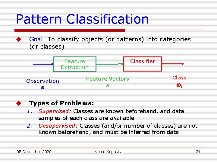
Pattern Classification u Goal: To classify objects (or patterns) into categories (or classes) Classifier Feature Extraction Observation Feature Vectors s u x Class i Types of Problems: 1. 2. Supervised: Classes are known beforehand, and data samples of each class are available Unsupervised: Classes (and/or number of classes) are not known beforehand, and must be inferred from data 05 December 2020 Veton Këpuska 24

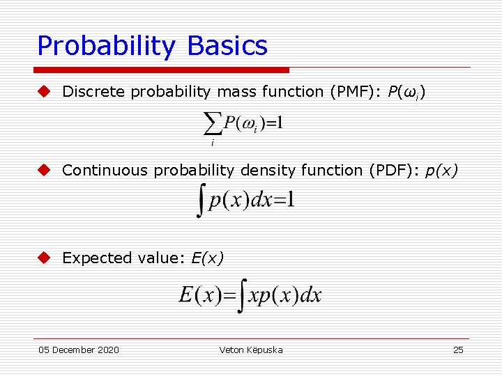
Probability Basics u Discrete probability mass function (PMF): P(ωi) u Continuous probability density function (PDF): p(x) u Expected value: E(x) 05 December 2020 Veton Këpuska 25

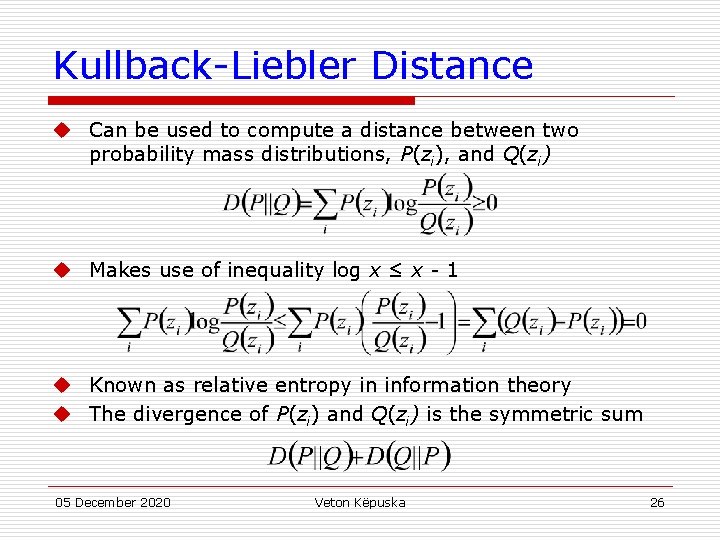
Kullback-Liebler Distance u Can be used to compute a distance between two probability mass distributions, P(zi), and Q(zi) u Makes use of inequality log x ≤ x - 1 u Known as relative entropy in information theory u The divergence of P(zi) and Q(zi) is the symmetric sum 05 December 2020 Veton Këpuska 26

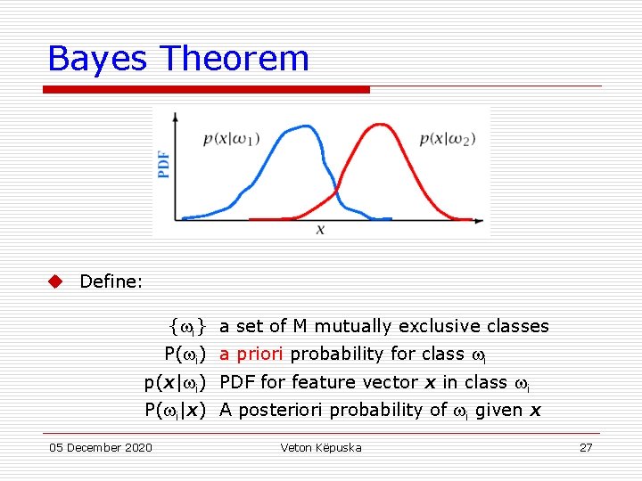
Bayes Theorem u Define: { i} a set of M mutually exclusive classes P( i) a priori probability for class i p(x| i) PDF for feature vector x in class i P( i|x) A posteriori probability of i given x 05 December 2020 Veton Këpuska 27

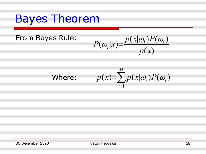
Bayes Theorem From Bayes Rule: Where: 05 December 2020 Veton Këpuska 28

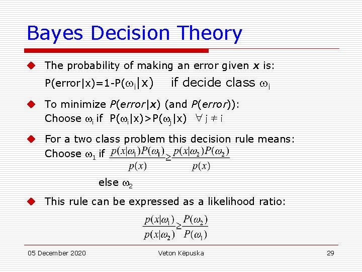
Bayes Decision Theory u The probability of making an error given x is: P(error|x)=1 -P( i|x) if decide class i u To minimize P(error|x) (and P(error)): Choose i if P( i|x)>P( j|x) ∀j≠i u For a two class problem this decision rule means: Choose 1 if else 2 u This rule can be expressed as a likelihood ratio: 05 December 2020 Veton Këpuska 29

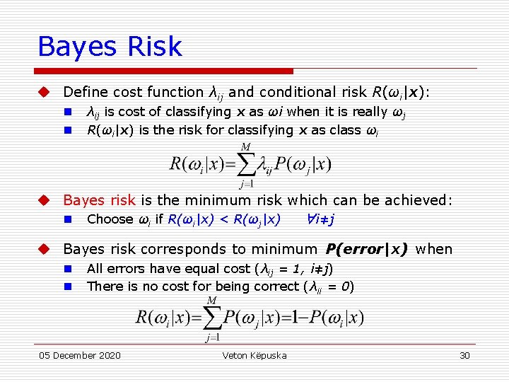
Bayes Risk u Define cost function λij and conditional risk R(ωi|x): n n λij is cost of classifying x as ωi when it is really ωj R(ωi|x) is the risk for classifying x as class ωi u Bayes risk is the minimum risk which can be achieved: n Choose ωi if R(ωi|x) < R(ωj|x) ∀i≠j u Bayes risk corresponds to minimum P(error|x) when n n All errors have equal cost (λij = 1, i≠j) There is no cost for being correct (λii = 0) 05 December 2020 Veton Këpuska 30

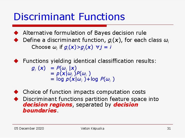
Discriminant Functions u Alternative formulation of Bayes decision rule u Define a discriminant function, gi(x), for each class ωi Choose ωi if gi(x)>gj(x) ∀j = i u Functions yielding identical classiffication results: gi (x) = P(ωi |x) = p(x|ωi )P(ωi ) = log p(x|ωi )+log P(ωi ) u Choice of function impacts computation costs u Discriminant functions partition feature space into decision regions, separated by decision boundaries. 05 December 2020 Veton Këpuska 31

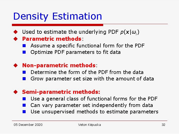
Density Estimation u Used to estimate the underlying PDF p(x|ωi) u Parametric methods: n Assume a specific functional form for the PDF n Optimize PDF parameters to fit data u Non-parametric methods: n Determine the form of the PDF from the data n Grow parameter set size with the amount of data u Semi-parametric methods: n Use a general class of functional forms for the PDF n Can vary parameter set independently from data n Use unsupervised methods to estimate parameters 05 December 2020 Veton Këpuska 32

Parametric Classifiers u Gaussian distributions u Maximum likelihood (ML) parameter estimation u Multivariate Gaussians u Gaussian classifiers 05 December 2020 Veton Këpuska 33

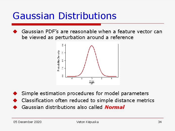
Gaussian Distributions u Gaussian PDF’s are reasonable when a feature vector can be viewed as perturbation around a reference u Simple estimation procedures for model parameters u Classification often reduced to simple distance metrics u Gaussian distributions also called Normal 05 December 2020 Veton Këpuska 34

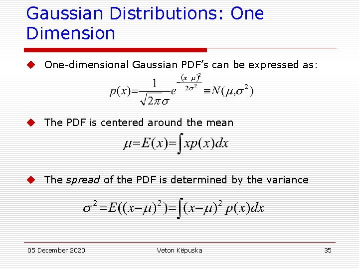
Gaussian Distributions: One Dimension u One-dimensional Gaussian PDF’s can be expressed as: u The PDF is centered around the mean u The spread of the PDF is determined by the variance 05 December 2020 Veton Këpuska 35

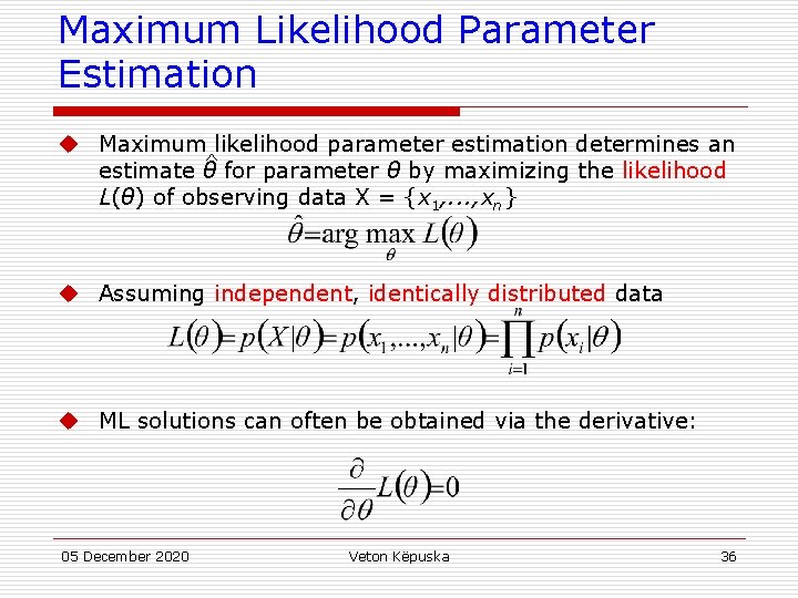
Maximum Likelihood Parameter Estimation u Maximum likelihood parameter estimation determines an ^ estimate θ for parameter θ by maximizing the likelihood L(θ) of observing data X = {x 1, . . . , xn} u Assuming independent, identically distributed data u ML solutions can often be obtained via the derivative: 05 December 2020 Veton Këpuska 36

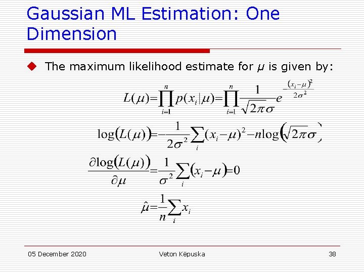
Maximum Likelihood Parameter Estimation u For Gaussian distributions log L(θ) is easier to solve 05 December 2020 Veton Këpuska 37

Gaussian ML Estimation: One Dimension u The maximum likelihood estimate for μ is given by: 05 December 2020 Veton Këpuska 38

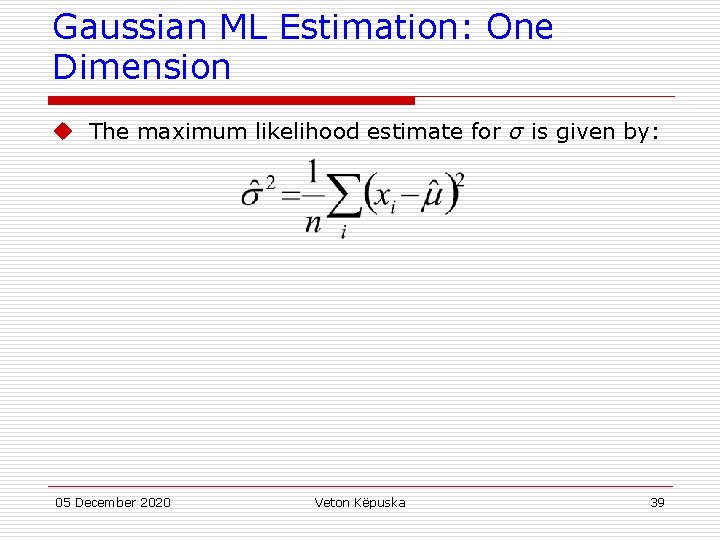
Gaussian ML Estimation: One Dimension u The maximum likelihood estimate for σ is given by: 05 December 2020 Veton Këpuska 39

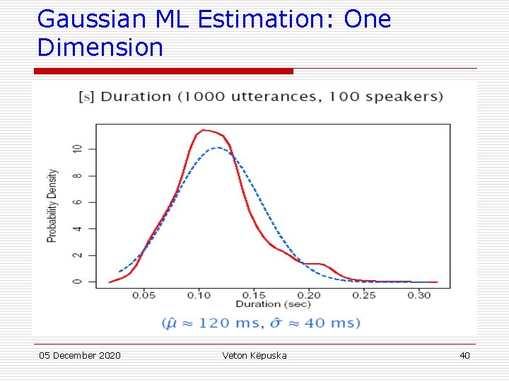
Gaussian ML Estimation: One Dimension 05 December 2020 Veton Këpuska 40

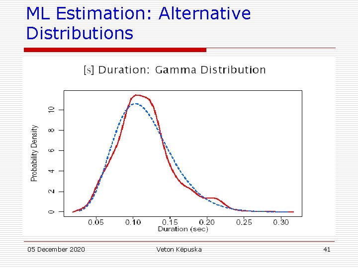
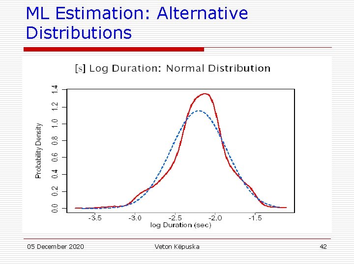
ML Estimation: Alternative Distributions 05 December 2020 Veton Këpuska 41

ML Estimation: Alternative Distributions 05 December 2020 Veton Këpuska 42

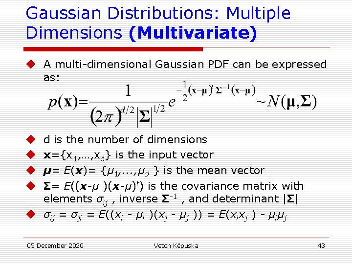
Gaussian Distributions: Multiple Dimensions (Multivariate) u A multi-dimensional Gaussian PDF can be expressed as: d is the number of dimensions x={x 1, …, xd} is the input vector μ= E(x)= {μ 1, . . . , μd } is the mean vector Σ= E((x-μ )(x-μ)t) is the covariance matrix with elements σij , inverse Σ-1 , and determinant |Σ| u σij = σji = E((xi - μi )(xj - μj )) = E(xixj ) - μiμj u u 05 December 2020 Veton Këpuska 43

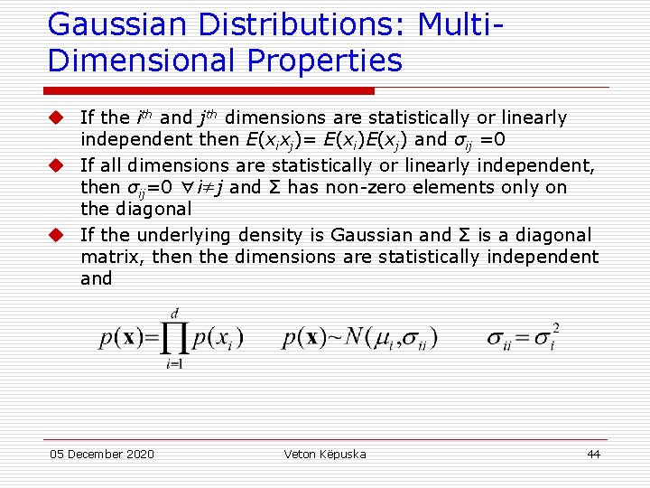
Gaussian Distributions: Multi. Dimensional Properties u If the ith and jth dimensions are statistically or linearly independent then E(xixj)= E(xi)E(xj) and σij =0 u If all dimensions are statistically or linearly independent, then σij=0 ∀i≠j and Σ has non-zero elements only on the diagonal u If the underlying density is Gaussian and Σ is a diagonal matrix, then the dimensions are statistically independent and 05 December 2020 Veton Këpuska 44

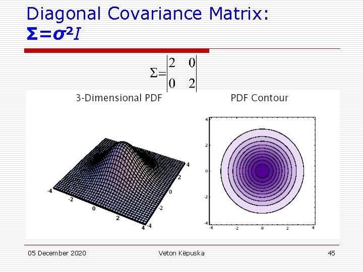
Diagonal Covariance Matrix: Σ=σ2 I 05 December 2020 Veton Këpuska 45

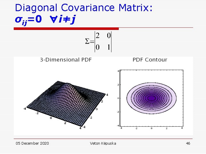
Diagonal Covariance Matrix: σij=0 ∀i≠j 05 December 2020 Veton Këpuska 46

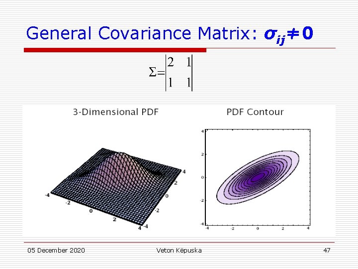
General Covariance Matrix: σij≠ 0 05 December 2020 Veton Këpuska 47

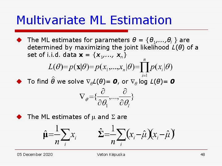
Multivariate ML Estimation u The ML estimates for parameters θ = {θ 1, . . . , θl } are determined by maximizing the joint likelihood L(θ) of a set of i. i. d. data x = {x 1, . . . , xn} ^ u To find θ we solve θL(θ)= 0, or θ log L(θ)= 0 u The ML estimates of and are 05 December 2020 Veton Këpuska 48

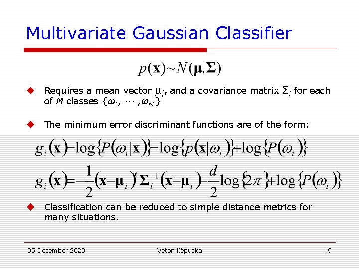
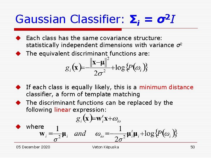
Multivariate Gaussian Classifier u Requires a mean vector i, and a covariance matrix Σi for each of M classes {ω1, ··· , ωM } u The minimum error discriminant functions are of the form: u Classification can be reduced to simple distance metrics for many situations. 05 December 2020 Veton Këpuska 49

Gaussian Classifier: Σi = σ2 I u Each class has the same covariance structure: statistically independent dimensions with variance σ2 u The equivalent discriminant functions are: u If each class is equally likely, this is a minimum distance classifier, a form of template matching u The discriminant functions can be replaced by the following linear expression: u where 05 December 2020 Veton Këpuska 50

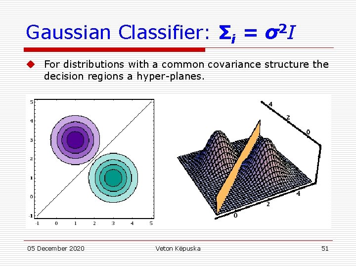
Gaussian Classifier: Σi = σ2 I u For distributions with a common covariance structure the decision regions a hyper-planes. 05 December 2020 Veton Këpuska 51

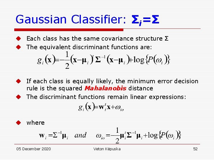
Gaussian Classifier: Σi=Σ u Each class has the same covariance structure Σ u The equivalent discriminant functions are: u If each class is equally likely, the minimum error decision rule is the squared Mahalanobis distance u The discriminant functions remain linear expressions: u where 05 December 2020 Veton Këpuska 52

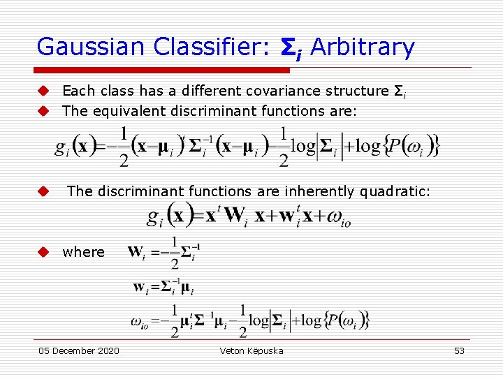
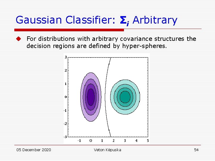
Gaussian Classifier: Σi Arbitrary u Each class has a different covariance structure Σ i u The equivalent discriminant functions are: u The discriminant functions are inherently quadratic: u where 05 December 2020 Veton Këpuska 53

Gaussian Classifier: Σi Arbitrary u For distributions with arbitrary covariance structures the decision regions are defined by hyper-spheres. 05 December 2020 Veton Këpuska 54

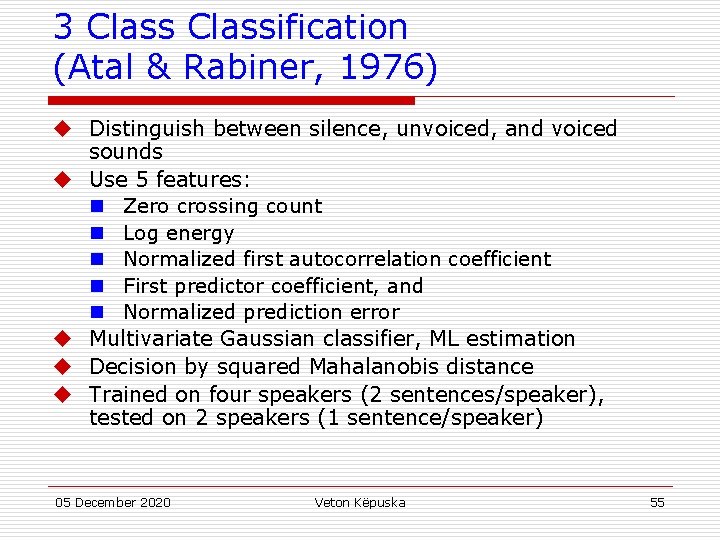
3 Classification (Atal & Rabiner, 1976) u Distinguish between silence, unvoiced, and voiced sounds u Use 5 features: n Zero crossing count n Log energy n Normalized first autocorrelation coefficient n First predictor coefficient, and n Normalized prediction error u Multivariate Gaussian classifier, ML estimation u Decision by squared Mahalanobis distance u Trained on four speakers (2 sentences/speaker), tested on 2 speakers (1 sentence/speaker) 05 December 2020 Veton Këpuska 55

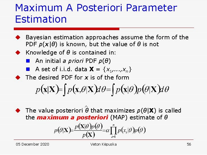
Maximum A Posteriori Parameter Estimation u Bayesian estimation approaches assume the form of the PDF p(x|θ) is known, but the value of θ is not u Knowledge of θ is contained in: n An initial a priori PDF p(θ) n A set of i. i. d. data X = {x 1, . . . , xn} u The desired PDF for x is of the form ^ u The value posteriori θ that maximizes p(θ|X) is called the maximum a posteriori (MAP) estimate of θ 05 December 2020 Veton Këpuska 56

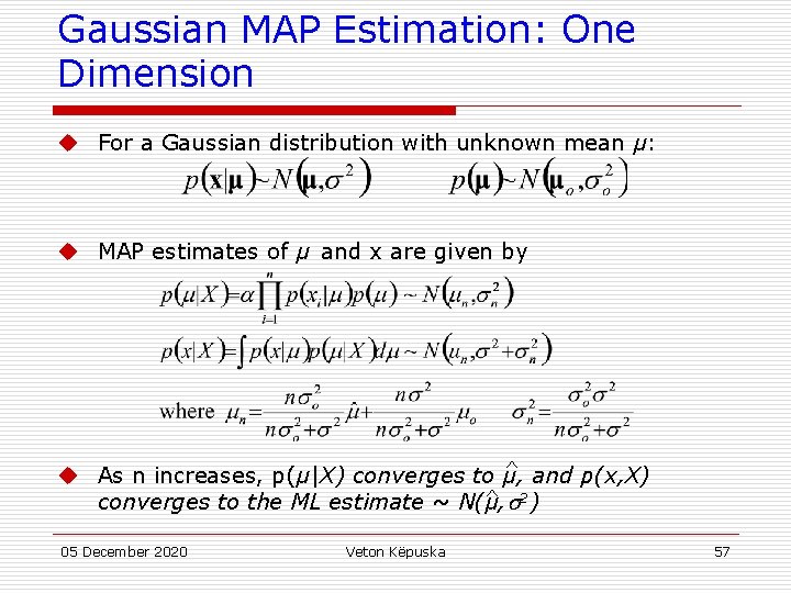
Gaussian MAP Estimation: One Dimension u For a Gaussian distribution with unknown mean μ: u MAP estimates of μ and x are given by ^ and p(x, X) u As n increases, p(μ|X) converges to μ, ^ 2) converges to the ML estimate ~ N(μ, 05 December 2020 Veton Këpuska 57

References u Huang, Acero, and Hon, Spoken Language Processing, Prentice-Hall, 2001. u Duda, Hart and Stork, Pattern Classification, John Wiley & Sons, 2001. u Atal and Rabiner, A Pattern Recognition Approach to Voiced-Unvoiced-Silence Classification with Applications to Speech Recognition, IEEE Trans ASSP, 24(3), 1976. 05 December 2020 Veton Këpuska 58

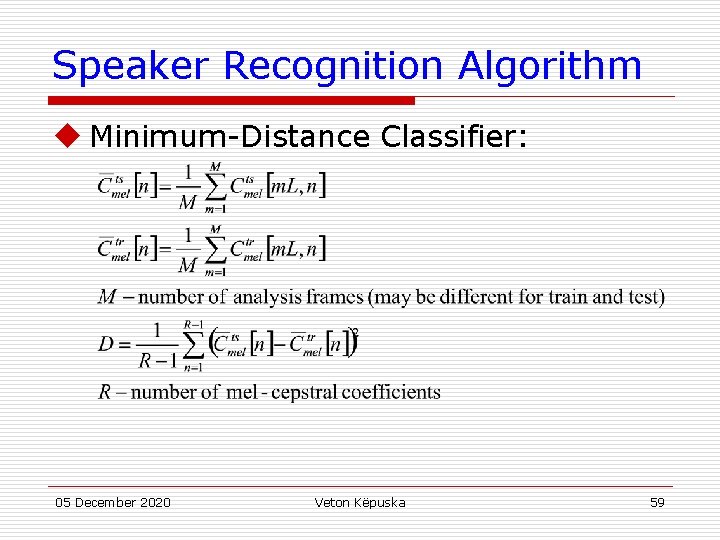
Speaker Recognition Algorithm u Minimum-Distance Classifier: 05 December 2020 Veton Këpuska 59

Vector Quantization u Class dependent Distance 05 December 2020 Veton Këpuska 60

Gaussian Mixture Model (GMM) u Speech Production not Deterministic: n Phones are never produced by a speaker with exactly the same vocal tract shape and glottal flow due to variations in: u Context u Coarticulation u Anatomy u Fluid Dynamics u On of the best ways to represent variability is through multi-dimensinal Gaussian pdf’s. u In general a Mixture of Gaussians is used to represent a class pdf. 05 December 2020 Veton Këpuska 61

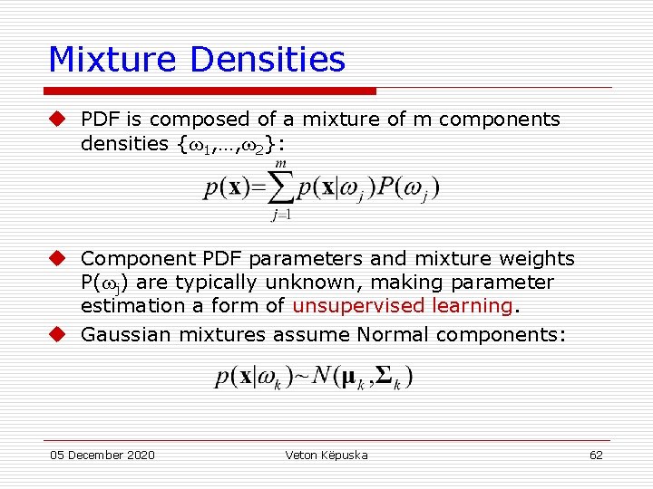
Mixture Densities u PDF is composed of a mixture of m components densities { 1, …, 2}: u Component PDF parameters and mixture weights P( j) are typically unknown, making parameter estimation a form of unsupervised learning. u Gaussian mixtures assume Normal components: 05 December 2020 Veton Këpuska 62

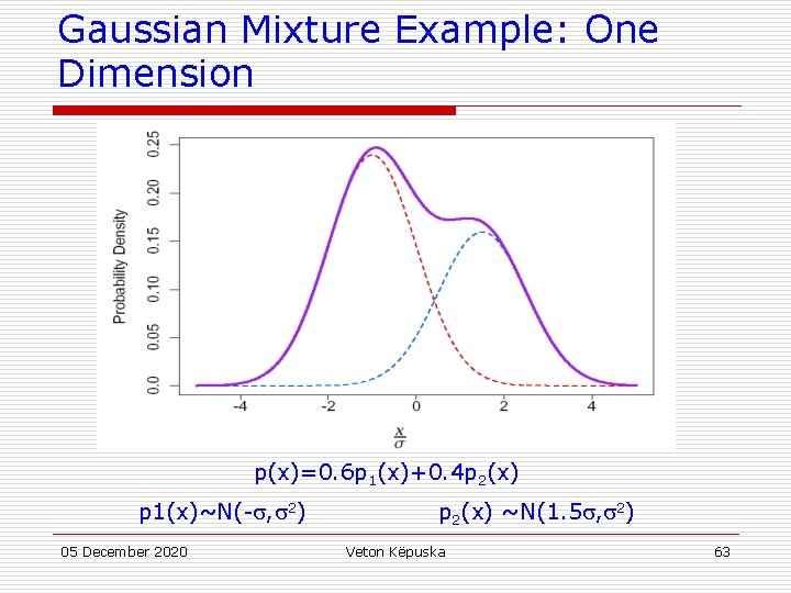
Gaussian Mixture Example: One Dimension p(x)=0. 6 p 1(x)+0. 4 p 2(x) p 1(x)~N(- , 2) 05 December 2020 p 2(x) ~N(1. 5 , 2) Veton Këpuska 63

Gaussian Example First 9 MFCC’s from [s]: Gaussian PDF 05 December 2020 Veton Këpuska 64

Independent Mixtures [s]: 2 Gaussian Mixture Components/Dimension 05 December 2020 Veton Këpuska 65

Mixture Components [s]: 2 Gaussian Mixture Components/Dimension 05 December 2020 Veton Këpuska 66

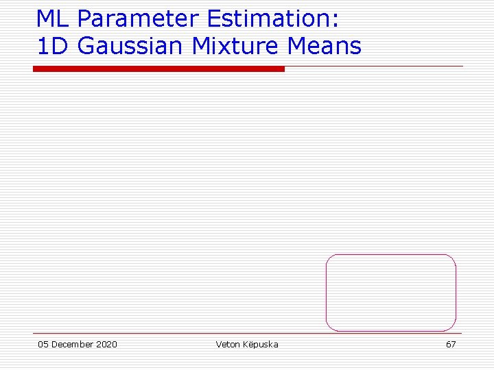
ML Parameter Estimation: 1 D Gaussian Mixture Means 05 December 2020 Veton Këpuska 67

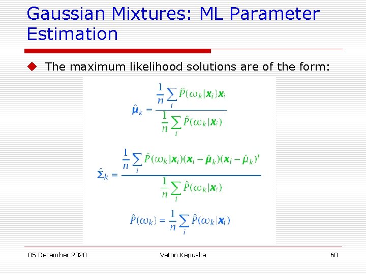
Gaussian Mixtures: ML Parameter Estimation u The maximum likelihood solutions are of the form: 05 December 2020 Veton Këpuska 68

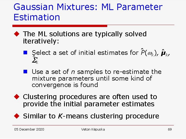
Gaussian Mixtures: ML Parameter Estimation u The ML solutions are typically solved iteratively: n Select a set of initial estimates for ˆ P( k), ˆ µk , ˆ k n Use a set of n samples to re-estimate the mixture parameters until some kind of convergence is found u Clustering procedures are often used to provide the initial parameter estimates u Similar to K-means clustering procedure 05 December 2020 Veton Këpuska 69

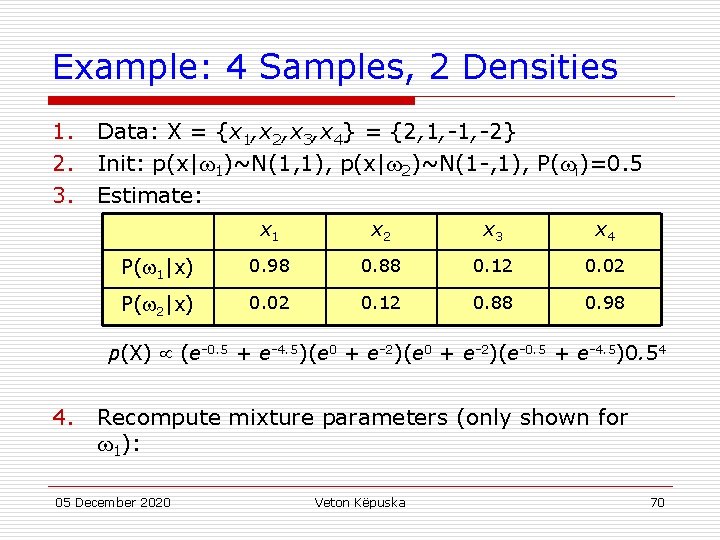
Example: 4 Samples, 2 Densities 1. 2. 3. Data: X = {x 1, x 2, x 3, x 4} = {2, 1, -2} Init: p(x| 1)~N(1, 1), p(x| 2)~N(1 -, 1), P( i)=0. 5 Estimate: x 1 x 2 x 3 x 4 P( 1|x) 0. 98 0. 88 0. 12 0. 02 P( 2|x) 0. 02 0. 12 0. 88 0. 98 p(X) (e-0. 5 + e-4. 5)(e 0 + e-2)(e-0. 5 + e-4. 5)0. 54 4. Recompute mixture parameters (only shown for 1): 05 December 2020 Veton Këpuska 70

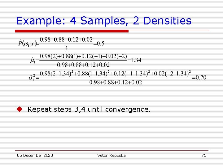
Example: 4 Samples, 2 Densities u Repeat steps 3, 4 until convergence. 05 December 2020 Veton Këpuska 71

[s] Duration: 2 Densities 05 December 2020 Veton Këpuska 72

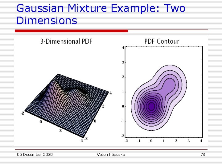
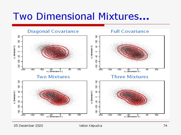
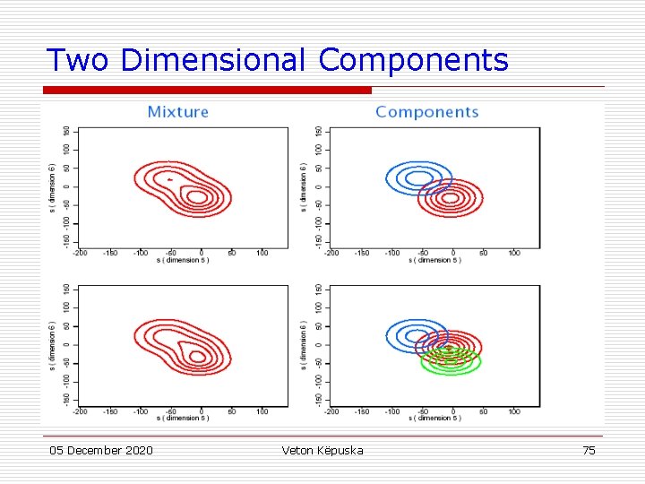
Gaussian Mixture Example: Two Dimensions 05 December 2020 Veton Këpuska 73

Two Dimensional Mixtures. . . 05 December 2020 Veton Këpuska 74

Two Dimensional Components 05 December 2020 Veton Këpuska 75

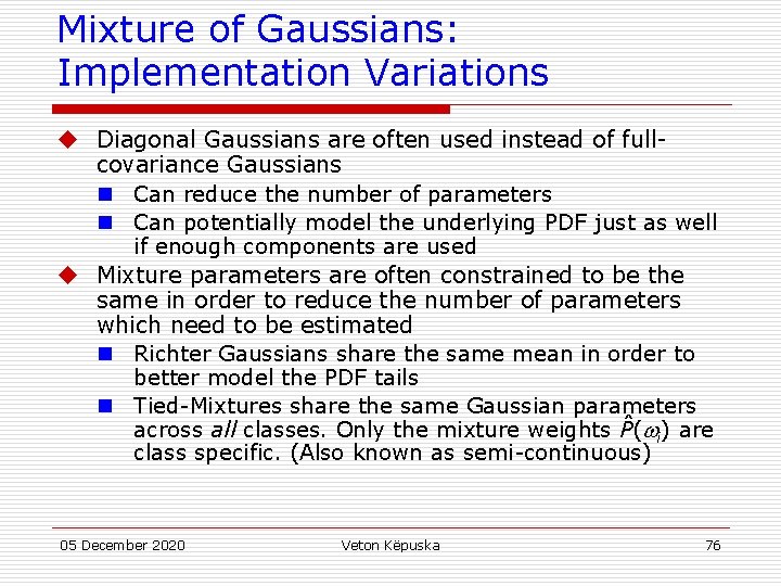
Mixture of Gaussians: Implementation Variations u Diagonal Gaussians are often used instead of fullcovariance Gaussians n Can reduce the number of parameters n Can potentially model the underlying PDF just as well if enough components are used u Mixture parameters are often constrained to be the same in order to reduce the number of parameters which need to be estimated n Richter Gaussians share the same mean in order to better model the PDF tails n Tied-Mixtures share the same Gaussian parameters ˆ i) are across all classes. Only the mixture weights P( class specific. (Also known as semi-continuous) 05 December 2020 Veton Këpuska 76

Richter Gaussian Mixtures u [s] Log Duration: 2 Richter Gaussians 05 December 2020 Veton Këpuska 77

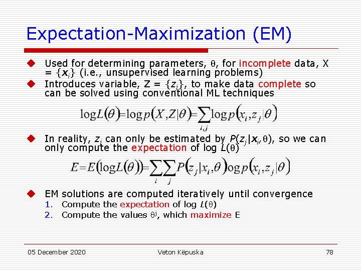
Expectation-Maximization (EM) u Used for determining parameters, , for incomplete data, X = {xi} (i. e. , unsupervised learning problems) u Introduces variable, Z = {zj}, to make data complete so can be solved using conventional ML techniques u In reality, zj can only be estimated by P(zj|xi, ), so we can only compute the expectation of log L( ) u EM solutions are computed iteratively until convergence 1. Compute the expectation of log L( ) 2. Compute the values j, which maximize E 05 December 2020 Veton Këpuska 78

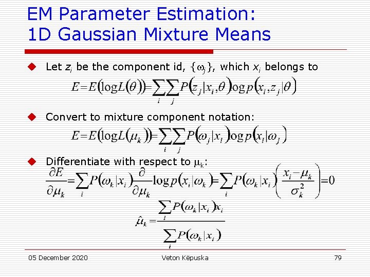
EM Parameter Estimation: 1 D Gaussian Mixture Means u Let zi be the component id, { j}, which xi belongs to u Convert to mixture component notation: u Differentiate with respect to k: 05 December 2020 Veton Këpuska 79

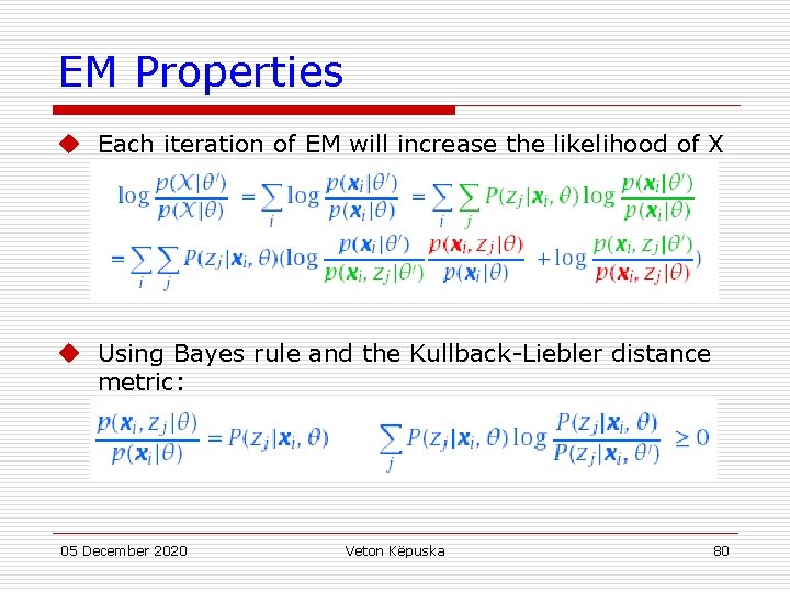
EM Properties u Each iteration of EM will increase the likelihood of X u Using Bayes rule and the Kullback-Liebler distance metric: 05 December 2020 Veton Këpuska 80

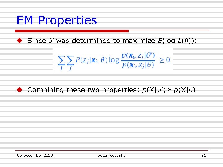
EM Properties u Since ’ was determined to maximize E(log L( )): u Combining these two properties: p(X| ’)≥ p(X| ) 05 December 2020 Veton Këpuska 81

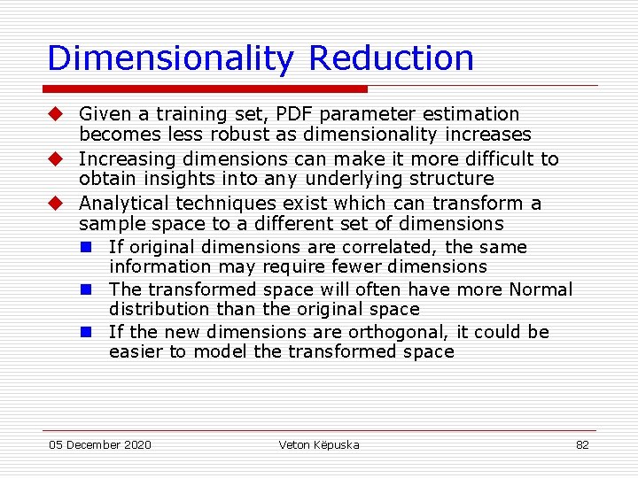
Dimensionality Reduction u Given a training set, PDF parameter estimation becomes less robust as dimensionality increases u Increasing dimensions can make it more difficult to obtain insights into any underlying structure u Analytical techniques exist which can transform a sample space to a different set of dimensions n If original dimensions are correlated, the same information may require fewer dimensions n The transformed space will often have more Normal distribution than the original space n If the new dimensions are orthogonal, it could be easier to model the transformed space 05 December 2020 Veton Këpuska 82

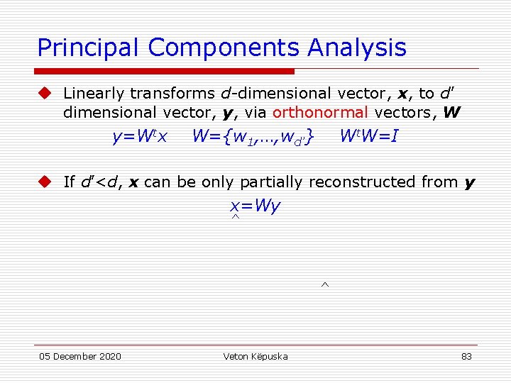
Principal Components Analysis u Linearly transforms d-dimensional vector, x, to d’ dimensional vector, y, via orthonormal vectors, W y=Wtx W={w 1, …, wd’} Wt. W=I u If d’<d, x can be only partially reconstructed from y x=Wy ^ ^ 05 December 2020 Veton Këpuska 83

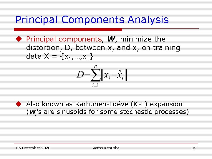
Principal Components Analysis u Principal components, W, minimize the distortion, D, between x, and x, on training data X = {x 1, …, xn} u Also known as Karhunen-Loéve (K-L) expansion (wi’s are sinusoids for some stochastic processes) 05 December 2020 Veton Këpuska 84

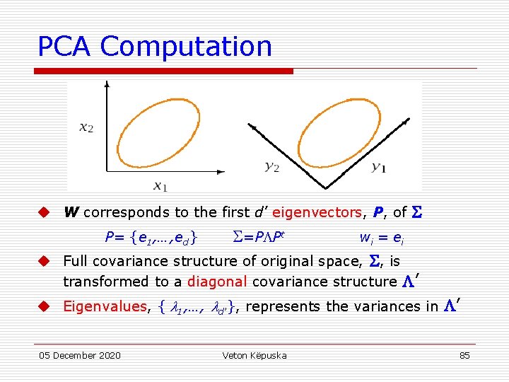
PCA Computation u W corresponds to the first d’ eigenvectors, P, of P= {e 1, …, ed} =P Pt wi = e i u Full covariance structure of original space, , is transformed to a diagonal covariance structure ’ u Eigenvalues, { 1, …, d’}, represents the variances in ’ 05 December 2020 Veton Këpuska 85

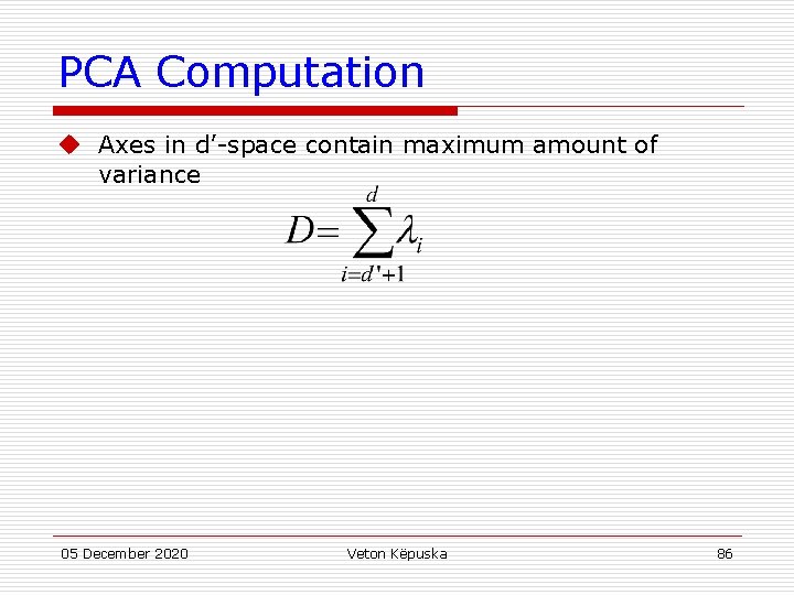
PCA Computation u Axes in d’-space contain maximum amount of variance 05 December 2020 Veton Këpuska 86

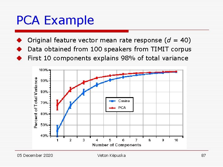
PCA Example u Original feature vector mean rate response (d = 40) u Data obtained from 100 speakers from TIMIT corpus u First 10 components explains 98% of total variance 05 December 2020 Veton Këpuska 87

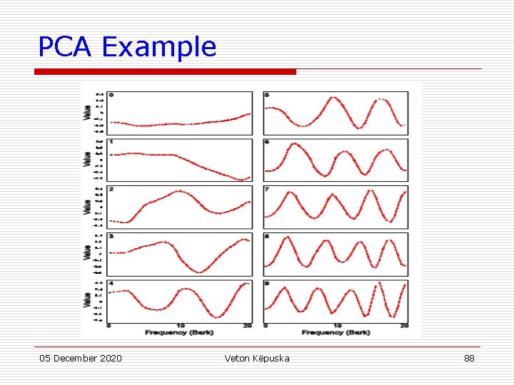
PCA Example 05 December 2020 Veton Këpuska 88

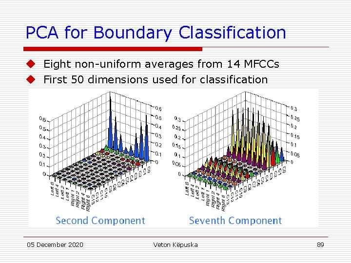
PCA for Boundary Classification u Eight non-uniform averages from 14 MFCCs u First 50 dimensions used for classification 05 December 2020 Veton Këpuska 89

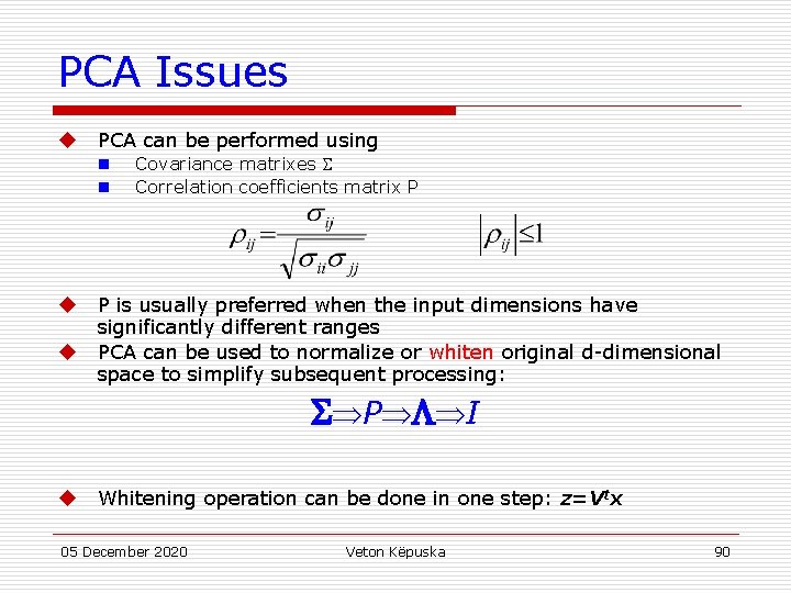
PCA Issues u PCA can be performed using n n u u Covariance matrixes Correlation coefficients matrix P P is usually preferred when the input dimensions have significantly different ranges PCA can be used to normalize or whiten original d-dimensional space to simplify subsequent processing: P I u Whitening operation can be done in one step: z=Vtx 05 December 2020 Veton Këpuska 90

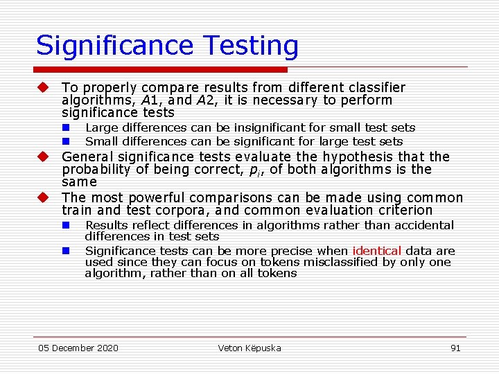
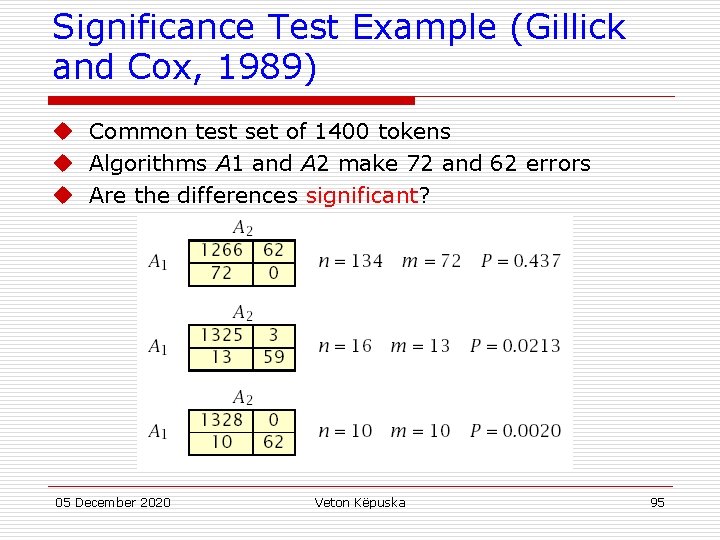
Significance Testing u To properly compare results from different classifier algorithms, A 1, and A 2, it is necessary to perform significance tests n n Large differences can be insignificant for small test sets Small differences can be significant for large test sets n Results reflect differences in algorithms rather than accidental differences in test sets Significance tests can be more precise when identical data are used since they can focus on tokens misclassified by only one algorithm, rather than on all tokens u General significance tests evaluate the hypothesis that the probability of being correct, pi, of both algorithms is the same u The most powerful comparisons can be made using common train and test corpora, and common evaluation criterion n 05 December 2020 Veton Këpuska 91

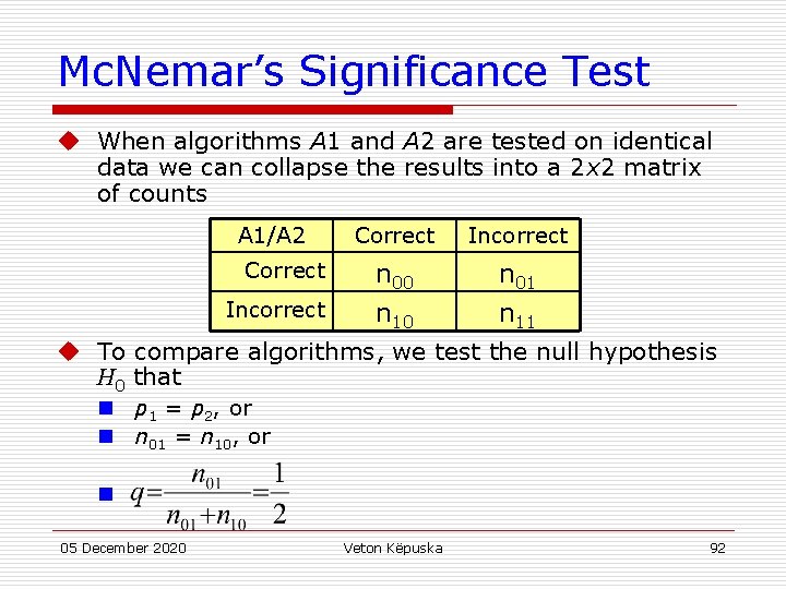
Mc. Nemar’s Significance Test u When algorithms A 1 and A 2 are tested on identical data we can collapse the results into a 2 x 2 matrix of counts A 1/A 2 Correct Incorrect Correct n 00 n 01 Incorrect n 10 n 11 u To compare algorithms, we test the null hypothesis H 0 that n p 1 = p 2, or n n 01 = n 10, or n 05 December 2020 Veton Këpuska 92

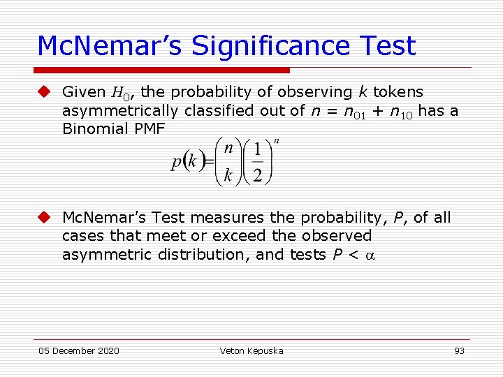
Mc. Nemar’s Significance Test u Given H 0, the probability of observing k tokens asymmetrically classified out of n = n 01 + n 10 has a Binomial PMF u Mc. Nemar’s Test measures the probability, P, of all cases that meet or exceed the observed asymmetric distribution, and tests P < 05 December 2020 Veton Këpuska 93

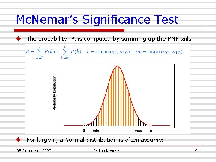
Mc. Nemar’s Significance Test u The probability, P, is computed by summing up the PMF tails u For large n, a Normal distribution is often assumed. 05 December 2020 Veton Këpuska 94

Significance Test Example (Gillick and Cox, 1989) u Common test set of 1400 tokens u Algorithms A 1 and A 2 make 72 and 62 errors u Are the differences significant? 05 December 2020 Veton Këpuska 95

References u Huang, Acero, and Hon, Spoken Language Processing, Prentice-Hall, 2001. u Duda, Hart and Stork, Pattern Classification, John Wiley & Sons, 2001. u Jelinek, Statistical Methods for Speech Recognition. MIT Press, 1997. u Bishop, Neural Networks for Pattern Recognition, Clarendon Press, 1995. u Gillick and Cox, Some Statistical Issues in the Comparison of Speech Recognition Algorithms, Proc. ICASSP, 1989. 05 December 2020 Veton Këpuska 96