Speech Processing Analysis and Synthesis of PoleZero Speech

Speech Processing Analysis and Synthesis of Pole-Zero Speech Models

Introduction u Deterministic: n Speech Sounds with periodic or impulse sources u Stochastic: n Speech Sounds with noise sources u Goal is to derive vocal tract model of each class of sound source. u It will be shown that solution equations for the two classes are similar in structure. u Solution approach is referred to as linear prediction analysis. n Linear prediction analysis leads to a method of speech synthesis based on the all-pole model. u Note that all-pole model is intimately associated with the concatenated lossless tube model of previous chapter (i. e. , Chapter 4). 11/4/2020 Veton Këpuska 2

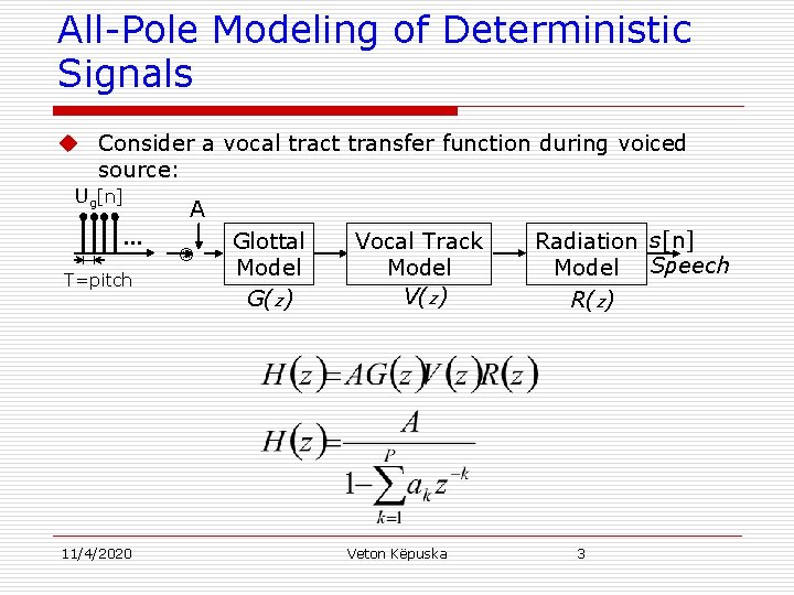
All-Pole Modeling of Deterministic Signals u Consider a vocal tract transfer function during voiced source: Ug[n] A … Glottal Vocal Track Radiation s[n] Model Speech T=pitch V(z) G(z) R(z) 11/4/2020 Veton Këpuska 3

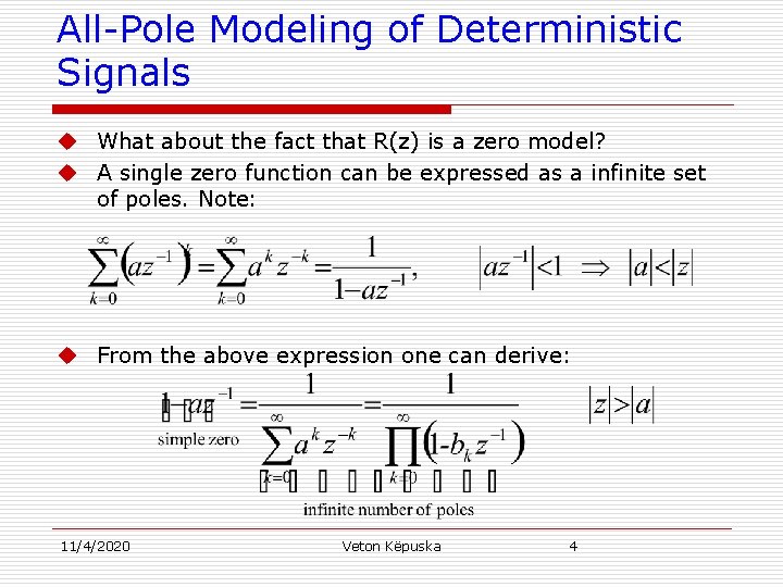
All-Pole Modeling of Deterministic Signals u What about the fact that R(z) is a zero model? u A single zero function can be expressed as a infinite set of poles. Note: u From the above expression one can derive: 11/4/2020 Veton Këpuska 4

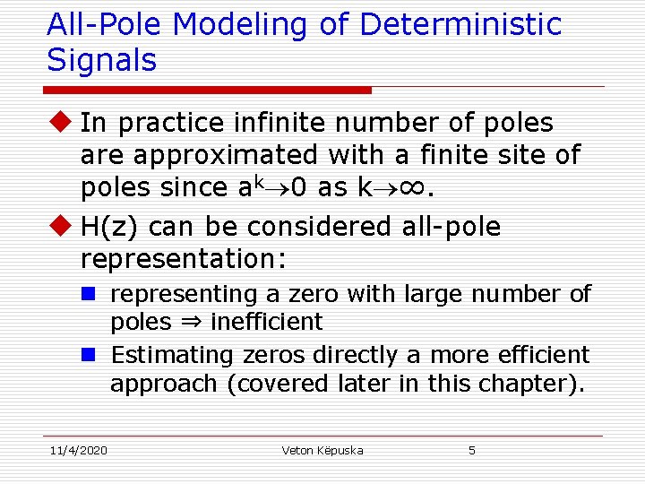
All-Pole Modeling of Deterministic Signals u In practice infinite number of poles are approximated with a finite site of poles since ak 0 as k ∞. u H(z) can be considered all-pole representation: n representing a zero with large number of poles ⇒ inefficient n Estimating zeros directly a more efficient approach (covered later in this chapter). 11/4/2020 Veton Këpuska 5

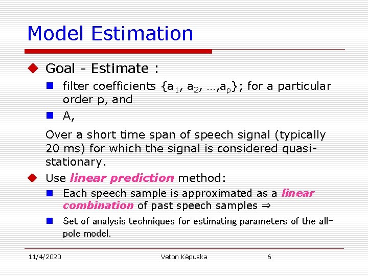
Model Estimation u Goal - Estimate : n filter coefficients {a 1, a 2, …, ap}; for a particular order p, and n A, Over a short time span of speech signal (typically 20 ms) for which the signal is considered quasistationary. u Use linear prediction method: n Each speech sample is approximated as a linear combination of past speech samples ⇒ n Set of analysis techniques for estimating parameters of the allpole model. 11/4/2020 Veton Këpuska 6

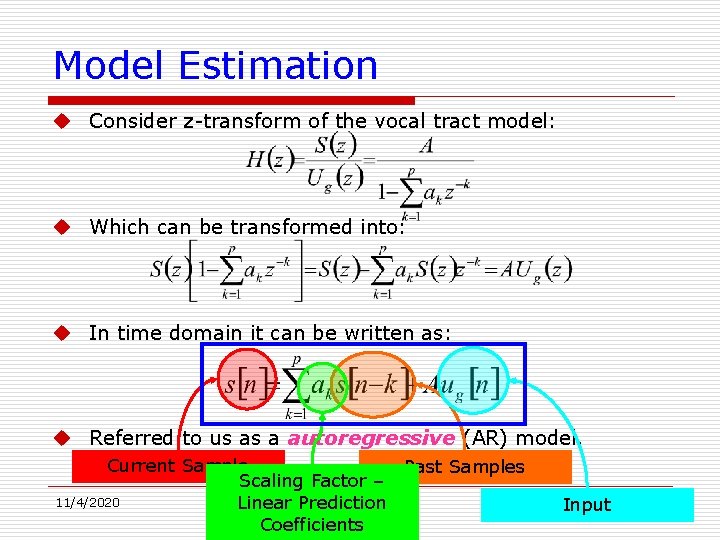
Model Estimation u Consider z-transform of the vocal tract model: u Which can be transformed into: u In time domain it can be written as: u Referred to us as a autoregressive (AR) model. Current Sample Past Samples Scaling Factor – 11/4/2020 Veton Këpuska 7 Linear Prediction Coefficients Input

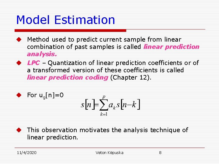
Model Estimation u Method used to predict current sample from linear combination of past samples is called linear prediction analysis. u LPC – Quantization of linear prediction coefficients or of a transformed version of these coefficients is called linear prediction coding (Chapter 12). u For ug[n]=0 u This observation motivates the analysis technique of linear prediction. 11/4/2020 Veton Këpuska 8

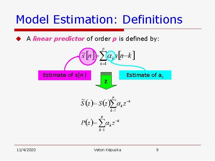
Model Estimation: Definitions u A linear predictor of order p is defined by: Estimate of s[n] 11/4/2020 z Veton Këpuska Estimate of ak 9

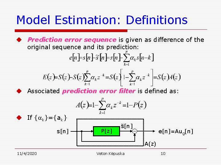
Model Estimation: Definitions u Prediction error sequence is given as difference of the original sequence and its prediction: u Associated prediction error filter is defined as: u If { k}={ak} s[n] P[z] s[n] ˜ e[n]=Aug[n] A(z) 11/4/2020 Veton Këpuska 10

Model Estimation: Definitions u Note 1: u Recovery of s[n]: Aug[n] 11/4/2020 s[n] Veton Këpuska 11

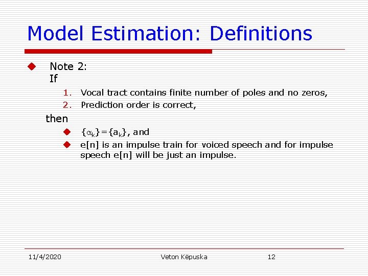
Model Estimation: Definitions u Note 2: If 1. Vocal tract contains finite number of poles and no zeros, 2. Prediction order is correct, then u { k}={ak}, and u e[n] is an impulse train for voiced speech and for impulse speech e[n] will be just an impulse. 11/4/2020 Veton Këpuska 12

Example 5. 1 u Consider an exponentially decaying impulse response of the form h[n]=anu[n] where u[n] is the unit step. Response to the scaled unit sample A [n] is: u Consider the prediction of s[n] using a linear predictor of order p=1. n It is a good fit since: n Prediction error sequence with 1=a is: n The prediction of the signal is exact except at the time origin. 11/4/2020 Veton Këpuska 13

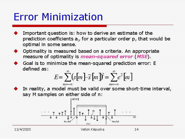
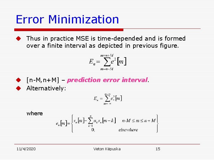
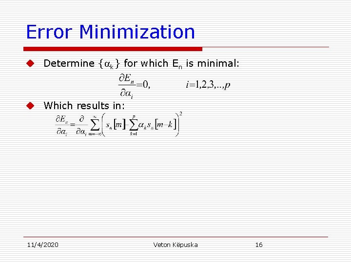
Error Minimization u u Important question is: how to derive an estimate of the prediction coefficients al, for a particular order p, that would be optimal in some sense. Optimality is measured based on a criteria. An appropriate measure of optimality is mean-squared error (MSE). Goal is to minimize the mean-squared prediction error: E defined as: In reality, a model must be valid over some short-time interval, say M samples on either side of n: 11/4/2020 Veton Këpuska 14

Error Minimization u Thus in practice MSE is time-depended and is formed over a finite interval as depicted in previous figure. u [n-M, n+M] – prediction error interval. u Alternatively: where 11/4/2020 Veton Këpuska 15

Error Minimization u Determine { k} for which En is minimal: u Which results in: 11/4/2020 Veton Këpuska 16

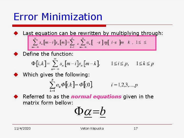
Error Minimization u Last equation can be rewritten by multiplying through: u Define the function: u Which gives the following: u Referred to as the normal equations given in the matrix form bellow: 11/4/2020 Veton Këpuska 17

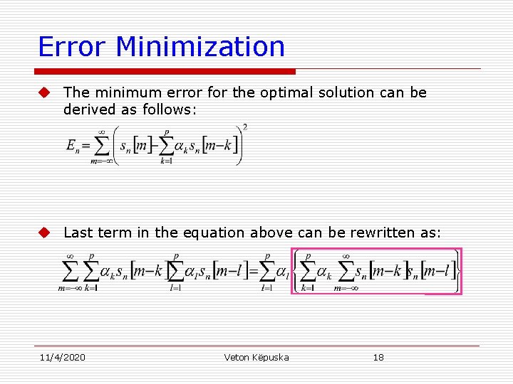
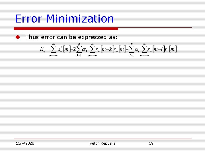
Error Minimization u The minimum error for the optimal solution can be derived as follows: u Last term in the equation above can be rewritten as: 11/4/2020 Veton Këpuska 18

Error Minimization u Thus error can be expressed as: 11/4/2020 Veton Këpuska 19

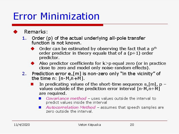
Error Minimization u Remarks: 1. Order (p) of the actual underlying all-pole transfer function is not known. u Order can be estimated by observing the fact that a pth u 2. order predictor in theory equals that of a (p+1) order predictor. Also predictor coefficients for k>p equal zero (or in practice close to zero and model only noise-random effects). Prediction error en[m] is non-zero only “in the vicinity” of the time n: [n-M, n+M]. n In predicating values of the short-time sequence sn[m], p – values outside of the prediction error interval [n-M, n+M] are required. n n 11/4/2020 Covariance method – uses values outside the interval to predict values inside the interval Autocorrelation Method – assumes that speech samples are zero outside the interval. Veton Këpuska 20

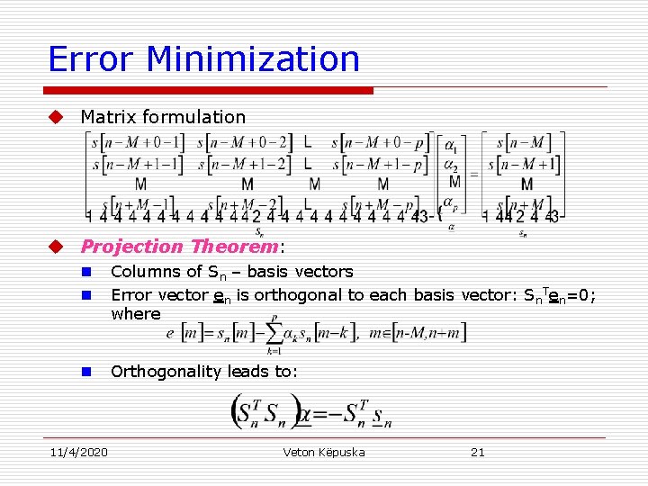
Error Minimization u Matrix formulation u Projection Theorem: n n Columns of Sn – basis vectors Error vector en is orthogonal to each basis vector: Sn. Ten=0; where n Orthogonality leads to: 11/4/2020 Veton Këpuska 21

Autocorrelation Method u In previous section we have described a general method of linear prediction that uses samples outside the prediction error interval referred to as covariance method. u Alternative approach that does not consider samples outside analysis interval, referred to as autocorrelation method, will be presented next. u This method is: n n 11/4/2020 Suboptimal, however it Leads to an efficient and stable solution to normal equations. Veton Këpuska 22

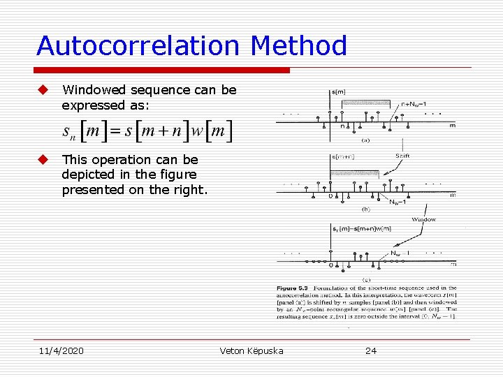
Autocorrelation Method u Assumes that the samples outside the time interval [n-M, n+M] are all zero, and u Extends the prediction error interval, i. e. , the range over which we minimize the mean-squared error to ±∞. u Conventions: n n Short-time interval: [n, n+Nw-1] where Nw=2 M+1 (Note: it is not centered around sample n as in previous derivation). Segment is shifted to the left by n samples so that the first nonzero sample falls at m=0. This operation is equivalent to: u Shifting of speech sequence s[m] by n-samples to the left and u Windowing by Nw -point rectangular window: 11/4/2020 Veton Këpuska 23

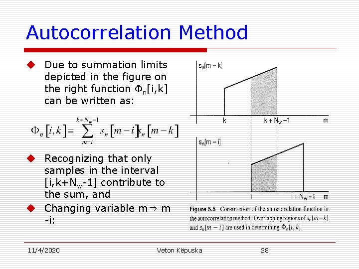
Autocorrelation Method u Windowed sequence can be expressed as: u This operation can be depicted in the figure presented on the right. 11/4/2020 Veton Këpuska 24

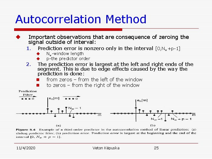
Autocorrelation Method u Important observations that are consequence of zeroing the signal outside of interval: 1. Prediction error is nonzero only in the interval [0, Nw+p-1] 2. 11/4/2020 u u Nw-window length p-the predictor order The prediction error is largest at the left and right ends of the segment. This is due to edge effects caused by the way the prediction is done: n from zeros – from the left of the window n to zeros – from the right of the window Veton Këpuska 25

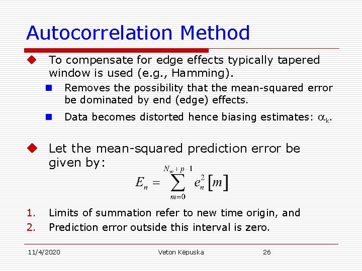
Autocorrelation Method u To compensate for edge effects typically tapered window is used (e. g. , Hamming). n Removes the possibility that the mean-squared error be dominated by end (edge) effects. n Data becomes distorted hence biasing estimates: u Let the mean-squared prediction error be given by: 1. 2. Limits of summation refer to new time origin, and Prediction error outside this interval is zero. 11/4/2020 Veton Këpuska 26 k.

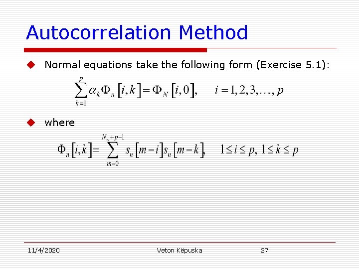
Autocorrelation Method u Normal equations take the following form (Exercise 5. 1): u where 11/4/2020 Veton Këpuska 27

Autocorrelation Method u Due to summation limits depicted in the figure on the right function n[i, k] can be written as: u Recognizing that only samples in the interval [i, k+Nw-1] contribute to the sum, and u Changing variable m⇒ m -i: 11/4/2020 Veton Këpuska 28

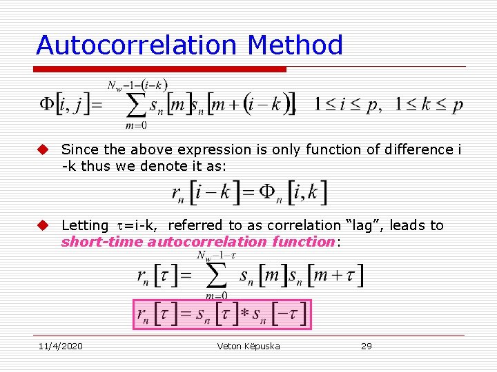
Autocorrelation Method u Since the above expression is only function of difference i -k thus we denote it as: u Letting =i-k, referred to as correlation “lag”, leads to short-time autocorrelation function: 11/4/2020 Veton Këpuska 29

Autocorrelation Method rn[ ]=sn[ ]*sn[- ] u Autocorrelation method leads to computation of the short-time sequence sn[m] convolved with itself flipped in time. u Autocorrelation function is a measure of the “self-similarity” of the signal at different lags . u When rn[ ] is large then signal samples spaced by are said to by highly correlated. 11/4/2020 Veton Këpuska 30

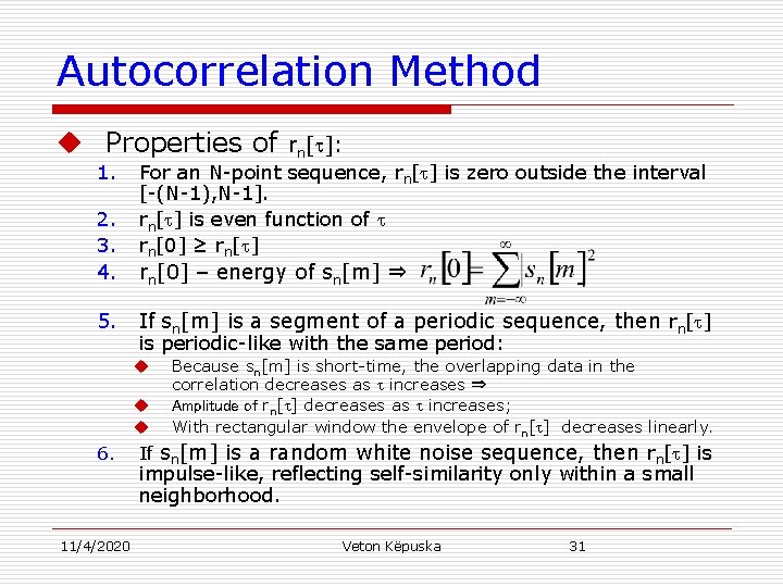
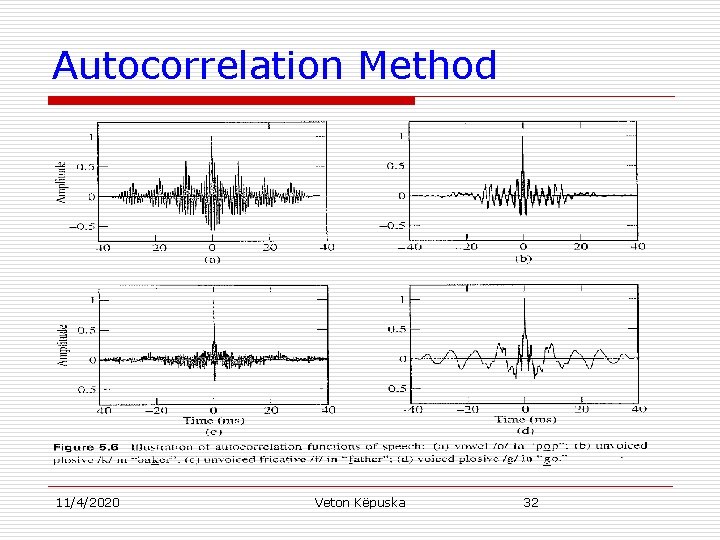
Autocorrelation Method u Properties of 1. 2. 3. 4. 5. For an N-point sequence, rn[ ] is zero outside the interval [-(N-1), N-1]. rn[ ] is even function of rn[0] ≥ rn[ ] rn[0] – energy of sn[m] ⇒ If sn[m] is a segment of a periodic sequence, then rn[ ] is periodic-like with the same period: u u u 6. 11/4/2020 rn[ ]: Because sn[m] is short-time, the overlapping data in the correlation decreases as increases ⇒ Amplitude of rn[ ] decreases as increases; With rectangular window the envelope of rn[ ] decreases linearly. If sn[m] is a random white noise sequence, then rn[ ] is impulse-like, reflecting self-similarity only within a small neighborhood. Veton Këpuska 31

Autocorrelation Method 11/4/2020 Veton Këpuska 32

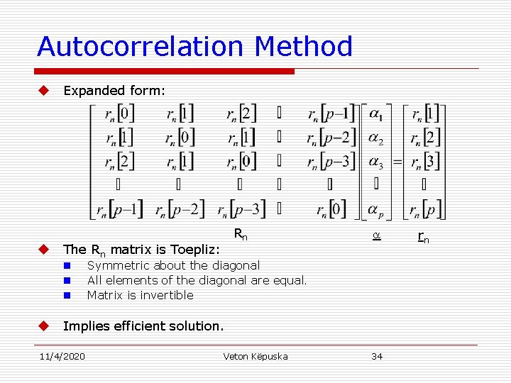
Autocorrelation Method u Letting n[i, k] = rn[i-k], normal equation take the form: u The expression represents p linear equations with p unknowns, k for 1≤k≤p. u Using the normal equation solution, it can be shown that the corresponding minimum mean-squared prediction error is given by: u Matrix form representation of normal equations: Rn =rn. 11/4/2020 Veton Këpuska 33

Autocorrelation Method u u Expanded form: The Rn matrix is Toepliz: n n n u Rn Symmetric about the diagonal All elements of the diagonal are equal. Matrix is invertible Implies efficient solution. 11/4/2020 Veton Këpuska 34 rn

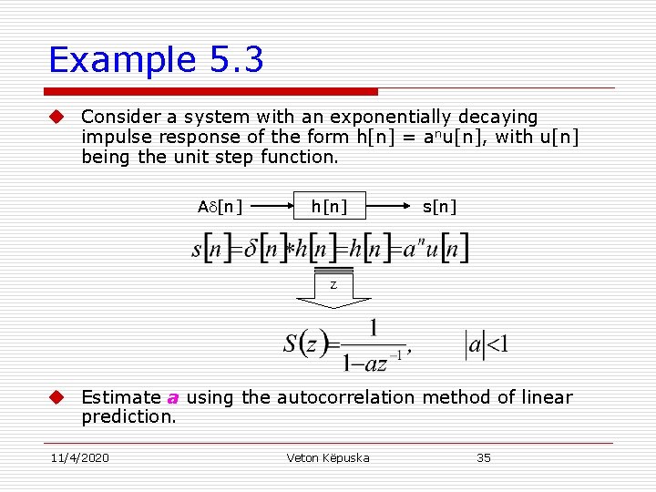
Example 5. 3 u Consider a system with an exponentially decaying impulse response of the form h[n] = anu[n], with u[n] being the unit step function. A [n] h[n] s[n] Z u Estimate a using the autocorrelation method of linear prediction. 11/4/2020 Veton Këpuska 35

Example 5. 3 u Apply N-point rectangular window [0, N-1] at n=0. u Compute r 0[0] and r 0[1]. u Using normal equations: 11/4/2020 Veton Këpuska 36

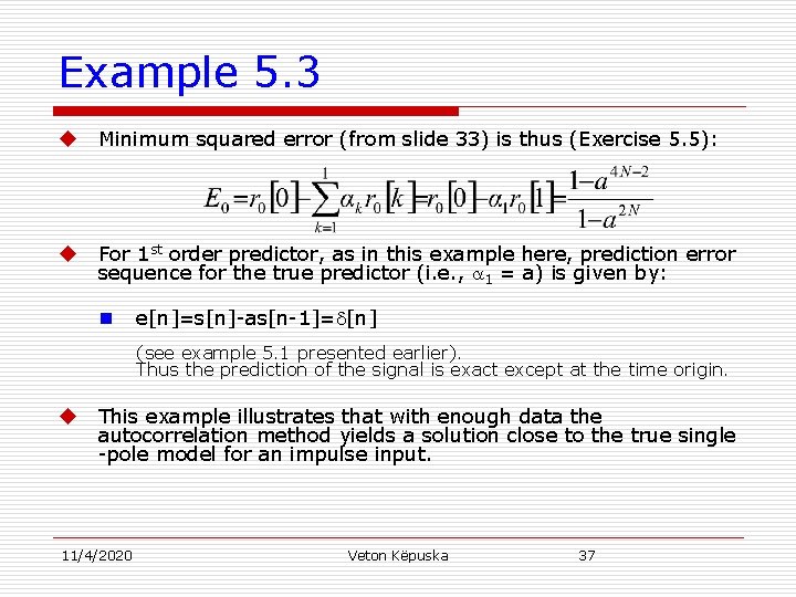
Example 5. 3 u Minimum squared error (from slide 33) is thus (Exercise 5. 5): u For 1 st order predictor, as in this example here, prediction error sequence for the true predictor (i. e. , 1 = a) is given by: n e[n]=s[n]-as[n-1]= [n] (see example 5. 1 presented earlier). Thus the prediction of the signal is exact except at the time origin. u This example illustrates that with enough data the autocorrelation method yields a solution close to the true single -pole model for an impulse input. 11/4/2020 Veton Këpuska 37

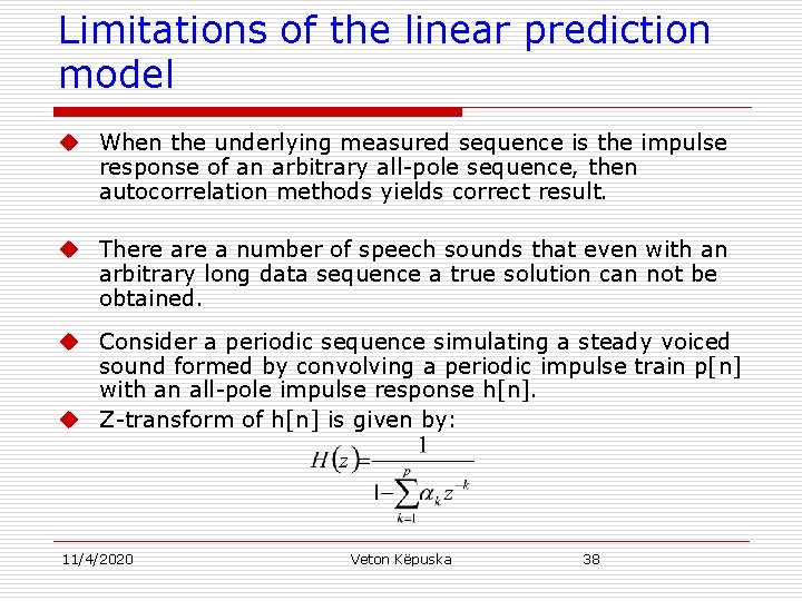
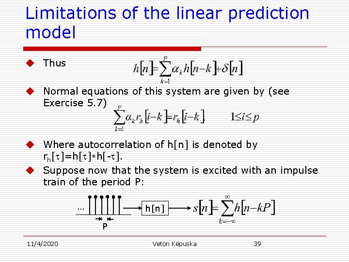
Limitations of the linear prediction model u When the underlying measured sequence is the impulse response of an arbitrary all-pole sequence, then autocorrelation methods yields correct result. u There a number of speech sounds that even with an arbitrary long data sequence a true solution can not be obtained. u Consider a periodic sequence simulating a steady voiced sound formed by convolving a periodic impulse train p[n] with an all-pole impulse response h[n]. u Z-transform of h[n] is given by: 11/4/2020 Veton Këpuska 38

Limitations of the linear prediction model u Thus u Normal equations of this system are given by (see Exercise 5. 7) u Where autocorrelation of h[n] is denoted by rh[ ]=h[ ]*h[- ]. u Suppose now that the system is excited with an impulse train of the period P: … h[n] P 11/4/2020 Veton Këpuska 39

Limitations of the linear prediction model u Normal equations associated with s[n] (windowed over multiple pitch periods) for an order p predictor are given by: u It can be shown that rn[ ] is equal to periodically repeated replicas of rh[ ]: but with decreasing amplitude due to the windowing (Exercise 5. 7). 11/4/2020 Veton Këpuska 40

Limitations of the linear prediction model u The autocorrelation function rn[ ] of the windowed signal s[n] can be thought of as “aliased” version of rh[ ] due to overlap which introduces distortion: 1. When aliasing is minor the two solutions are approximately equal. Accuracy of this approximation decreases as the pitch period decreases (e. g. , high pitch) due to increase in overlap of autocorrelation replicas repeated every P samples. 2. 11/4/2020 Veton Këpuska 41

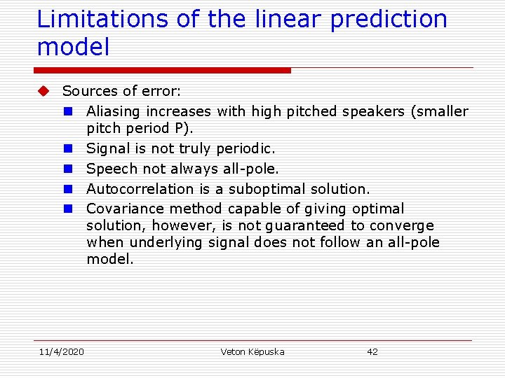
Limitations of the linear prediction model u Sources of error: n Aliasing increases with high pitched speakers (smaller pitch period P). n Signal is not truly periodic. n Speech not always all-pole. n Autocorrelation is a suboptimal solution. n Covariance method capable of giving optimal solution, however, is not guaranteed to converge when underlying signal does not follow an all-pole model. 11/4/2020 Veton Këpuska 42

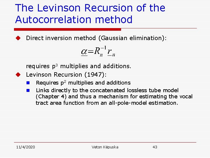
The Levinson Recursion of the Autocorrelation method u Direct inversion method (Gaussian elimination): requires p 3 multiplies and additions. u Levinson Recursion (1947): n n 11/4/2020 Requires p 2 multiplies and additions Links directly to the concatenated lossless tube model (Chapter 4) and thus a mechanism for estimating the vocal tract area function from an all-pole-model estimation. Veton Këpuska 43

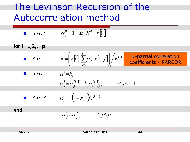
The Levinson Recursion of the Autocorrelation method n Step 1: for i=1, 2, …, p n Step 2: n Step 3: n Step 4: ki-partial correlation coefficients - PARCOR end 11/4/2020 Veton Këpuska 44

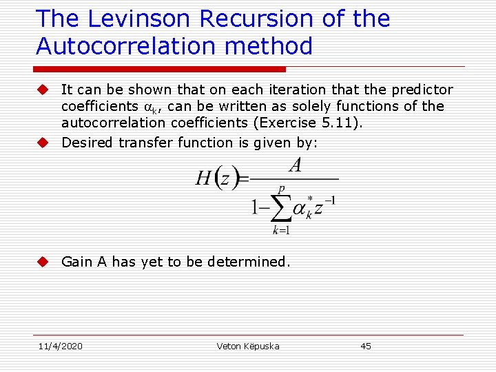
The Levinson Recursion of the Autocorrelation method u It can be shown that on each iteration that the predictor coefficients k, can be written as solely functions of the autocorrelation coefficients (Exercise 5. 11). u Desired transfer function is given by: u Gain A has yet to be determined. 11/4/2020 Veton Këpuska 45

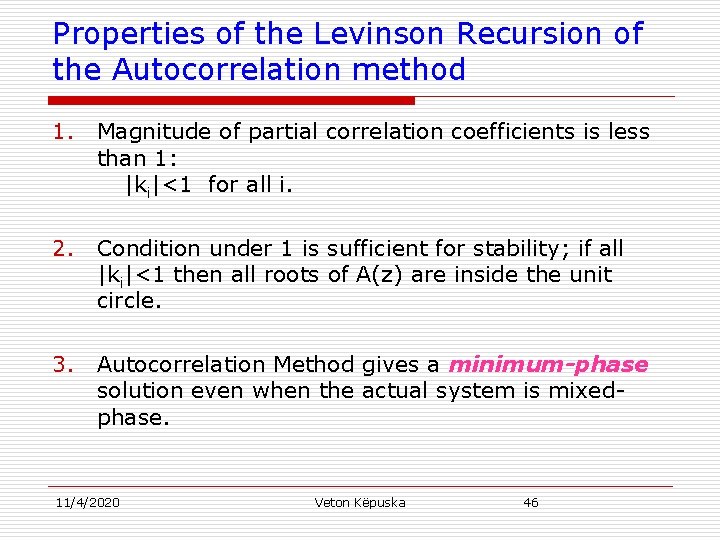
Properties of the Levinson Recursion of the Autocorrelation method 1. Magnitude of partial correlation coefficients is less than 1: |ki|<1 for all i. 2. Condition under 1 is sufficient for stability; if all |ki|<1 then all roots of A(z) are inside the unit circle. 3. Autocorrelation Method gives a minimum-phase solution even when the actual system is mixedphase. 11/4/2020 Veton Këpuska 46

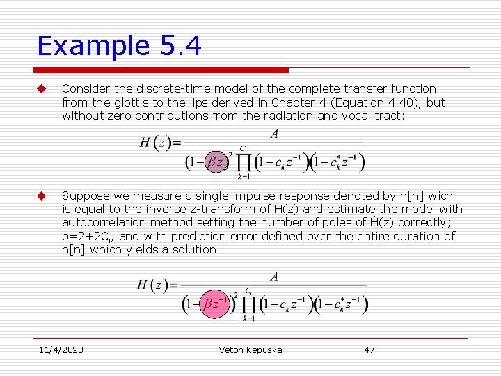
Example 5. 4 u Consider the discrete-time model of the complete transfer function from the glottis to the lips derived in Chapter 4 (Equation 4. 40), but without zero contributions from the radiation and vocal tract: u Suppose we measure a single impulse response denoted by h[n] wich is equal to the inverse z-transform of H(z) and estimate the model with autocorrelation method setting the number of poles of Ĥ(z) correctly; p=2+2 Ci, and with prediction error defined over the entire duration of h[n] which yields a solution 11/4/2020 Veton Këpuska 47

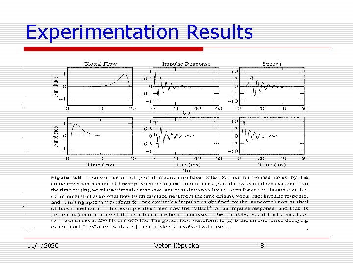
Experimentation Results 11/4/2020 Veton Këpuska 48

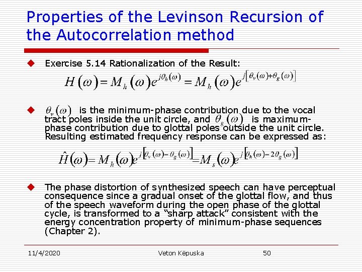
Properties of the Levinson Recursion of the Autocorrelation method Formal explanation: u Suppose s[n] follows an all-pole model u Prediction error function is defined over all time (i. e. , no window truncation effects: and are the Fourier transform phase functions for the minimum- and maximum-phase contributions of S( ), respectively. u Autocorrelation solution can be expressed as (Exercise 5. 14): u 11/4/2020 Veton Këpuska 49

Properties of the Levinson Recursion of the Autocorrelation method u Exercise 5. 14 Rationalization of the Result: u is the minimum-phase contribution due to the vocal tract poles inside the unit circle, and is maximumphase contribution due to glottal poles outside the unit circle. Resulting estimated frequency response can be expressed as: u The phase distortion of synthesized speech can have perceptual consequence since a gradual onset of the glottal flow, and thus of the speech waveform during the open phase of the glottal cycle, is transformed to a “sharp attack” consistent with the energy concentration property of minimum-phase sequences (Chapter 2). 11/4/2020 Veton Këpuska 50

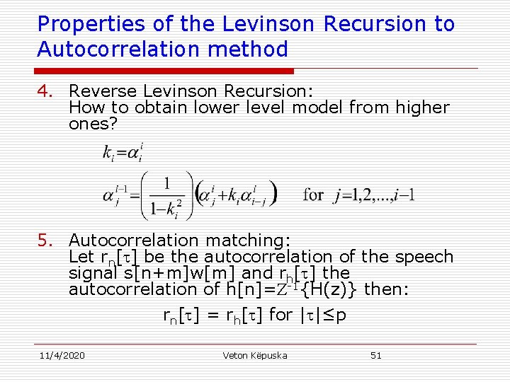
Properties of the Levinson Recursion to Autocorrelation method 4. Reverse Levinson Recursion: How to obtain lower level model from higher ones? 5. Autocorrelation matching: Let rn[ ] be the autocorrelation of the speech signal s[n+m]w[m] and rh[ ] the autocorrelation of h[n]= -1{H(z)} then: rn[ ] = rh[ ] for | |≤p 11/4/2020 Veton Këpuska 51

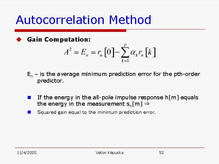
Autocorrelation Method u Gain Computation: En – is the average minimum prediction error for the pth-order predictor. n n 11/4/2020 If the energy in the all-pole impulse response h[m] equals the energy in the measurement sn[m] ⇒ Squared gain equal to the minimum prediction error. Veton Këpuska 52

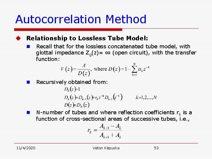
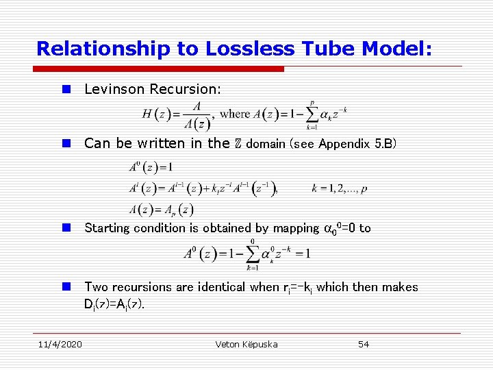
Autocorrelation Method u Relationship to Lossless Tube Model: n Recall that for the lossless concatenated tube model, with glottal impedance Zg(z)= ∞ (open circuit), with the transfer function: n Recursively obtained from: n N-number of tubes and where reflection coefficients r k is a function of cross-sectional areas of successive tubes, i. e. , 11/4/2020 Veton Këpuska 53

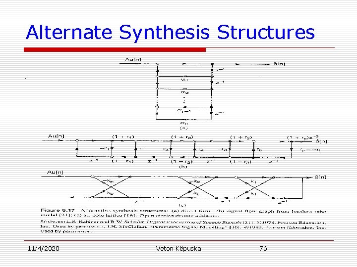
Relationship to Lossless Tube Model: n Levinson Recursion: n Can be written in the ℤ domain (see Appendix 5. B) n Starting condition is obtained by mapping 00=0 to n Two recursions are identical when ri=-ki which then makes Di(z)=Ai(z). 11/4/2020 Veton Këpuska 54

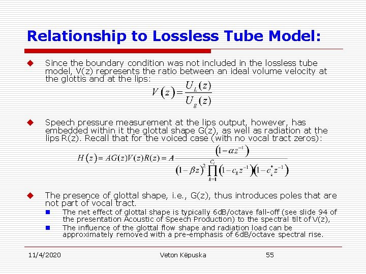
Relationship to Lossless Tube Model: u Since the boundary condition was not included in the lossless tube model, V(z) represents the ratio between an ideal volume velocity at the glottis and at the lips: u Speech pressure measurement at the lips output, however, has embedded within it the glottal shape G(z), as well as radiation at the lips R(z). Recall that for the voiced case (with no vocal tract zeros): u The presence of glottal shape, i. e. , G(z), thus introduces poles that are not part of vocal tract. n n 11/4/2020 The net effect of glottal shape is typically 6 d. B/octave fall-off (see slide 94 of the presentation Acoustic of Speech Production) to the spectral tilt of V(z), The influence of the glottal flow shape and radiation load can be approximately removed with a pre-emphasis of 6 d. B/octave spectral rise. Veton Këpuska 55

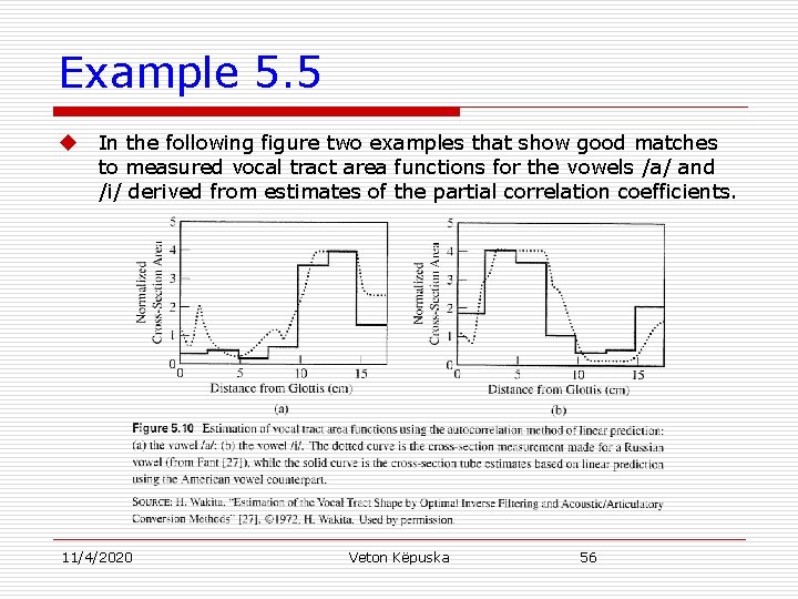
Example 5. 5 u In the following figure two examples that show good matches to measured vocal tract area functions for the vowels /a/ and /i/ derived from estimates of the partial correlation coefficients. 11/4/2020 Veton Këpuska 56

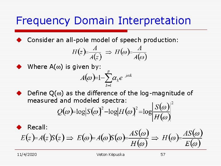
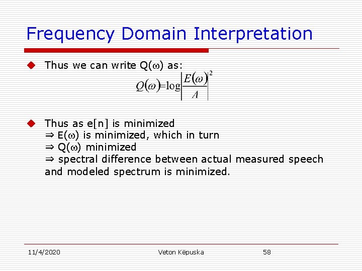
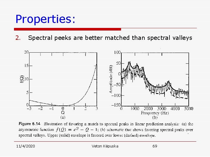
Frequency Domain Interpretation u Consider an all-pole model of speech production: u Where A( ) is given by: u Define Q( ) as the difference of the log-magnitude of measured and modeled spectra: u Recall: 11/4/2020 Veton Këpuska 57

Frequency Domain Interpretation u Thus we can write Q( ) as: u Thus as e[n] is minimized ⇒ E( ) is minimized, which in turn ⇒ Q( ) minimized ⇒ spectral difference between actual measured speech and modeled spectrum is minimized. 11/4/2020 Veton Këpuska 58

Linear Prediction Analysis of Stochastic Speech Sounds u Linear Prediction analysis was motivated with observation that for a single impulse or periodic impulse train input to an all-pole vocal tract model, the prediction error is zero “most of the time”. u Such analysis appears not to be applicable to speech sounds with fricative or aspirated sources modeled as a stochastic (or random) process. u However, autocorrelation method of linear prediction can be formulated for the stochastic case where a white noise input takes on the role of the single impulse. u The solution to a stochastic optimization problem - analogous to the minimization of mean-squared error function En, leads to normal equations which are the stochastic counterparts to our earlier solution. u Derivation and interpretation of this stochastic optimization problem is left as an exercise. 11/4/2020 Veton Këpuska 59

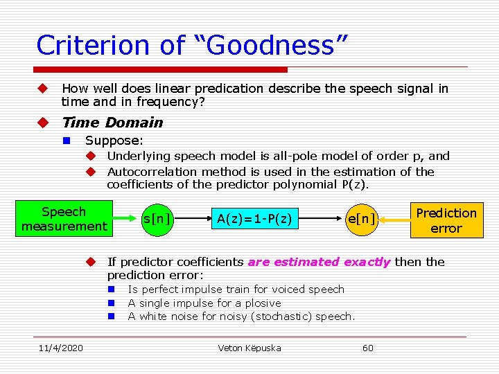
Criterion of “Goodness” u How well does linear predication describe the speech signal in time and in frequency? u Time Domain n Suppose: u Underlying speech model is all-pole model of order p, and u Autocorrelation method is used in the estimation of the coefficients of the predictor polynomial P(z). Speech measurement s[n] A(z)=1 -P(z) e[n] Prediction error u If predictor coefficients are estimated exactly then the prediction error: n n n 11/4/2020 Is perfect impulse train for voiced speech A single impulse for a plosive A white noise for noisy (stochastic) speech. Veton Këpuska 60

Time Domain u Autocorrelation method of linear prediction analysis does not yield such idealized outputs when the measurement s[n] is inverse filtered by the estimated system function A(z) (method limitation): n n Even when the vocal tract response follow an all-pole model, true solution can not be obtained, since the obtained solution approached to the true solution in the limit when infinite amount of data is available. In a typical waveform segment, the actual vocal tract impulse response is not all-pole for variety of reasons: u Presence of zeros due to: n n n The radiation load, Nasalization, Back vocal cavity during frication and plosives. u Glottal flow shape – even when adequately modeled, is not minimum phase (see example 5. 6). 11/4/2020 Veton Këpuska 61

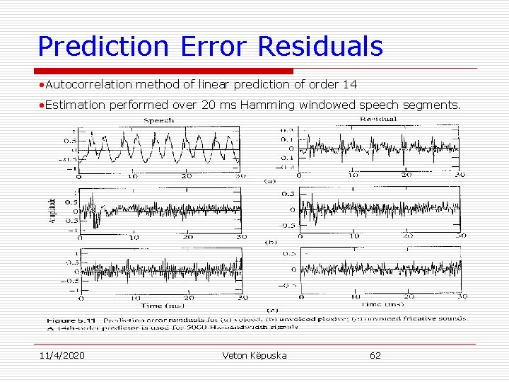
Prediction Error Residuals • Autocorrelation method of linear prediction of order 14 • Estimation performed over 20 ms Hamming windowed speech segments. 11/4/2020 Veton Këpuska 62

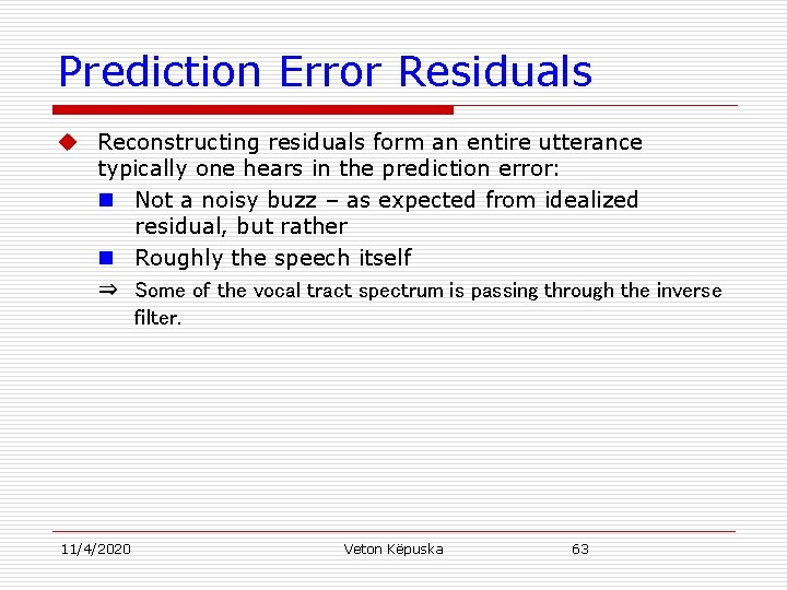
Prediction Error Residuals u Reconstructing residuals form an entire utterance typically one hears in the prediction error: n Not a noisy buzz – as expected from idealized residual, but rather n Roughly the speech itself ⇒ Some of the vocal tract spectrum is passing through the inverse filter. 11/4/2020 Veton Këpuska 63

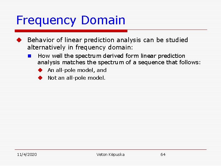
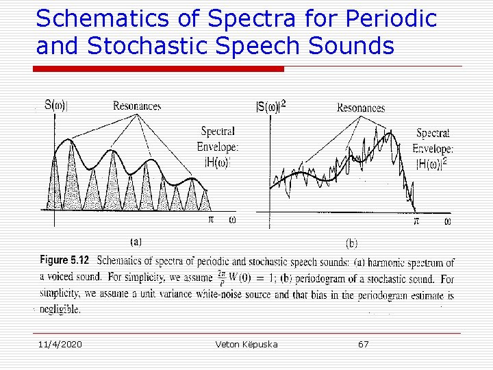
Frequency Domain u Behavior of linear prediction analysis can be studied alternatively in frequency domain: n 11/4/2020 How well the spectrum derived form linear prediction analysis matches the spectrum of a sequence that follows: u An all-pole model, and u Not an all-pole model. Veton Këpuska 64

Frequency Domain-Voiced Speech u Recall for voiced speech s[n]: with Fourier transform Ug( ). u Vocal tract impulse response with all-pole frequency response H( ). Windowed speech sn[n] is: u Fourier transform of windowed speech sn[n] is: u Where: n n 11/4/2020 W( ) o=2 /P - is the window transform - is the fundamental frequency Veton Këpuska 65

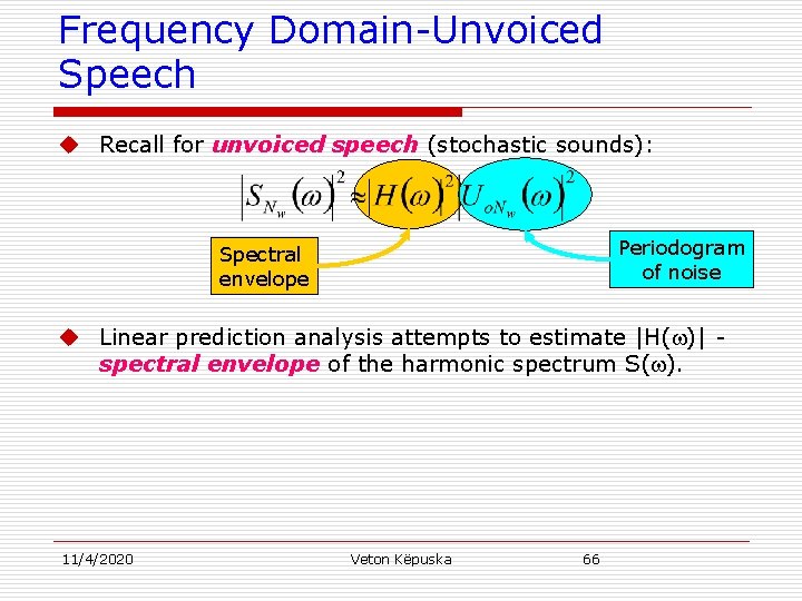
Frequency Domain-Unvoiced Speech u Recall for unvoiced speech (stochastic sounds): Periodogram of noise Spectral envelope u Linear prediction analysis attempts to estimate |H( )| spectral envelope of the harmonic spectrum S( ). 11/4/2020 Veton Këpuska 66

Schematics of Spectra for Periodic and Stochastic Speech Sounds 11/4/2020 Veton Këpuska 67

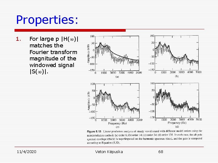
Properties: 1. For large p |H( )| matches the Fourier transform magnitude of the windowed signal |S( )|. 11/4/2020 Veton Këpuska 68

Properties: 2. Spectral peeks are better matched than spectral valleys 11/4/2020 Veton Këpuska 69

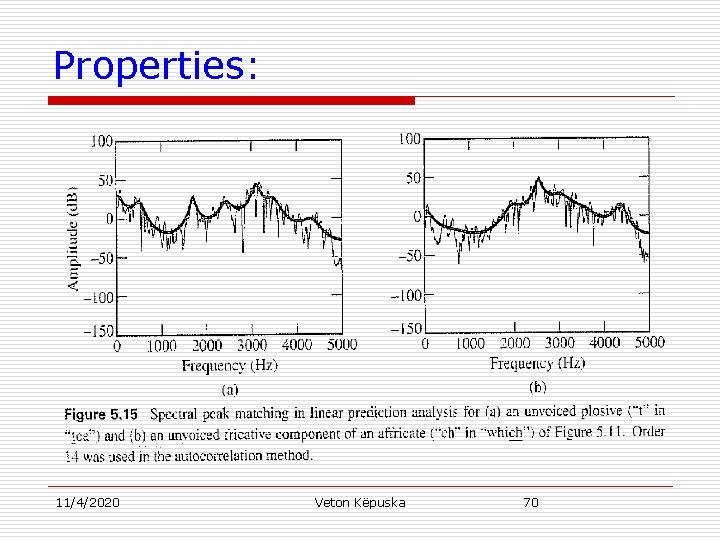
Properties: 11/4/2020 Veton Këpuska 70

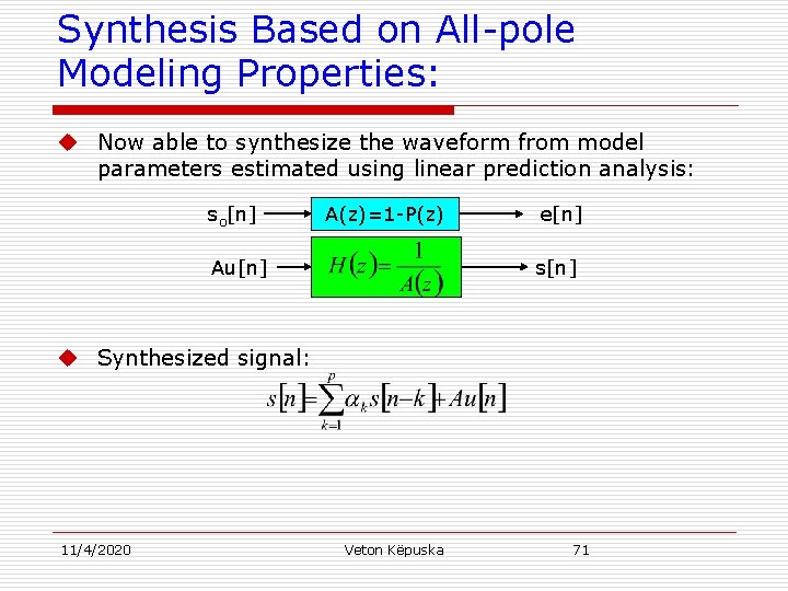
Synthesis Based on All-pole Modeling Properties: u Now able to synthesize the waveform from model parameters estimated using linear prediction analysis: so[n] A(z)=1 -P(z) Au[n] e[n] s[n] u Synthesized signal: 11/4/2020 Veton Këpuska 71

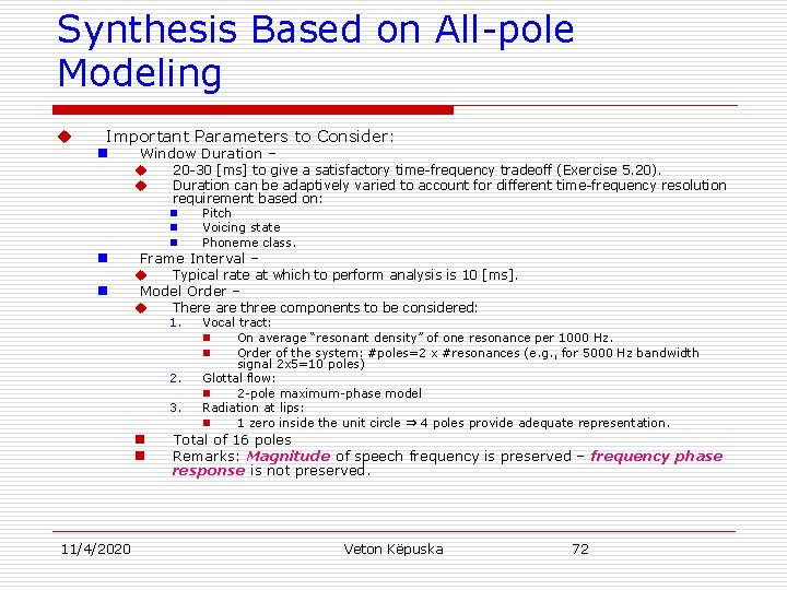
Synthesis Based on All-pole Modeling u Important Parameters to Consider: n Window Duration – u 20 -30 [ms] to give a satisfactory time-frequency tradeoff (Exercise 5. 20). u Duration can be adaptively varied to account for different time-frequency resolution requirement based on: n Pitch n Voicing state n Phoneme class. n n Frame Interval – u Typical rate at which to perform analysis is 10 [ms]. Model Order – u There are three components to be considered: 1. 2. 3. n n 11/4/2020 Vocal tract: n On average “resonant density” of one resonance per 1000 Hz. n Order of the system: #poles=2 x #resonances (e. g. , for 5000 Hz bandwidth signal 2 x 5=10 poles) Glottal flow: n 2 -pole maximum-phase model Radiation at lips: n 1 zero inside the unit circle ⇒ 4 poles provide adequate representation. Total of 16 poles Remarks: Magnitude of speech frequency is preserved – frequency phase response is not preserved. Veton Këpuska 72

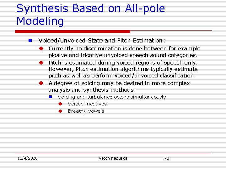
Synthesis Based on All-pole Modeling n Voiced/Unvoiced State and Pitch Estimation: u Currently no discrimination is done between for example plosive and fricative unvoiced speech sound categories. u Pitch is estimated during voiced regions of speech only. However, Pitch estimation algorithms typically estimate pitch as well as perform voiced/unvoiced classification. u A degree of voicing may be desired in more complex analysis and synthesis methods: n 11/4/2020 Voicing and turbulence occurs simultaneously u Voiced fricatives u Breathy vowels. Veton Këpuska 73

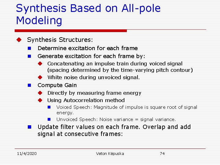
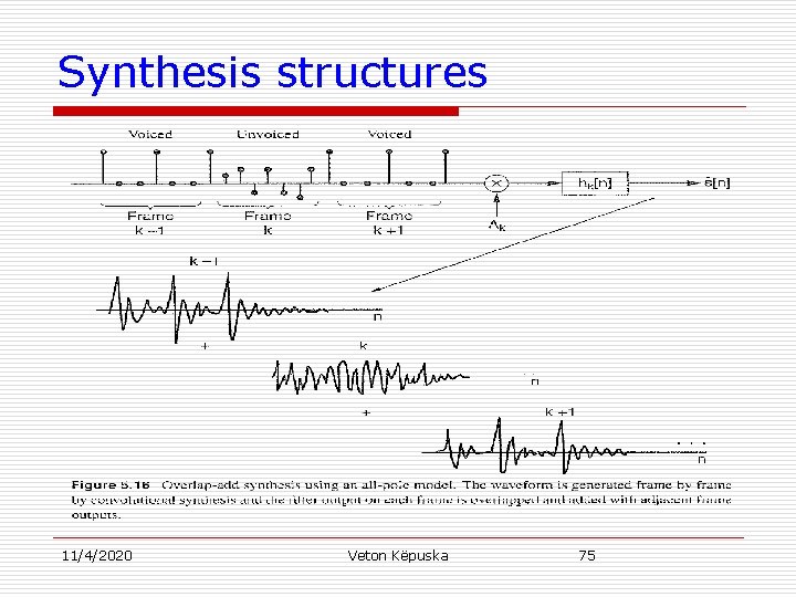
Synthesis Based on All-pole Modeling u Synthesis Structures: n n Determine excitation for each frame Generate excitation for each frame by: u Concatenating an impulse train during voiced signal (spacing determined by the time-varying pitch contour) u White noise during unvoiced signal. n Compute Gain u Directly by measuring frame energy u Using Autocorrelation method n n n 11/4/2020 Voiced Speech: Magnitude of impulse is square root of signal energy. Unvoiced Speech: Noise variance = signal variance. Update filter values on each frame. Overlap and add signal at consecutive frames: Veton Këpuska 74

Synthesis structures 11/4/2020 Veton Këpuska 75

Alternate Synthesis Structures 11/4/2020 Veton Këpuska 76