Specification of a CRM model Ken Cheung Department

Specification of a CRM model Ken Cheung Department of Biostatistics, Columbia University (joint work with Shing Lee @ Columbia)

Agenda • Motivation • Components of a CRM model – Dose-toxicity function – Initial guesses of DLT rates – Prior distribution of model parameter • Example: A bortezomib trial CRM Workshop October 2009

Motivation • The CRM is a model-based dose-finding method • Advantage (versus algorithmic designs): a coherent approach to contingencies via the model, e. g. , 1/3 + 0/3 + 1/1 …? • Assumption: The model specification is “good” • Practical problem: Specifying a CRM model can be a complex process … even for statisticians. CRM Workshop October 2009

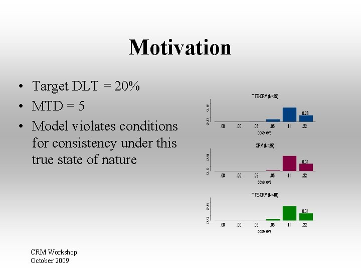
Motivation • Target DLT = 20% • MTD = 5 • Model violates conditions for consistency under this true state of nature CRM Workshop October 2009

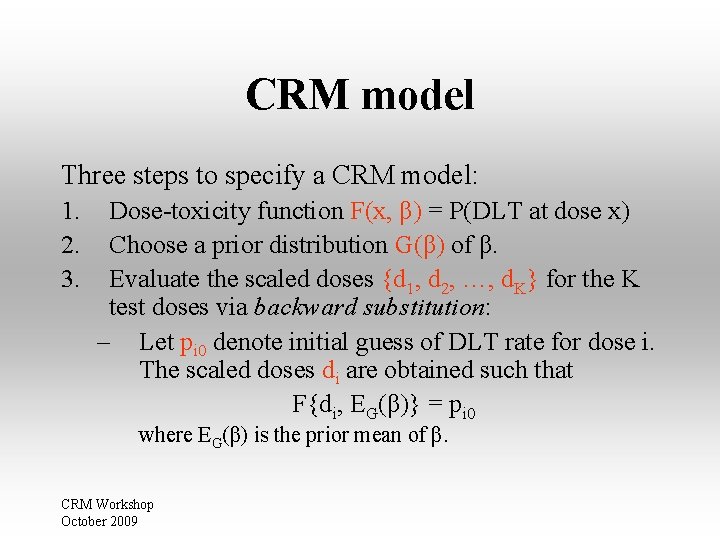
CRM model Three steps to specify a CRM model: 1. 2. 3. Dose-toxicity function F(x, β) = P(DLT at dose x) Choose a prior distribution G(β) of β. Evaluate the scaled doses {d 1, d 2, …, d. K} for the K test doses via backward substitution: – Let pi 0 denote initial guess of DLT rate for dose i. The scaled doses di are obtained such that F{di, EG(β)} = pi 0 where EG(β) is the prior mean of β. CRM Workshop October 2009

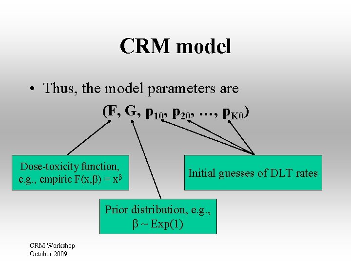
CRM model • Thus, the model parameters are (F, G, p 10, p 20, …, p. K 0) Dose-toxicity function, e. g. , empiric F(x, β) = xβ Initial guesses of DLT rates Prior distribution, e. g. , β ~ Exp(1) CRM Workshop October 2009

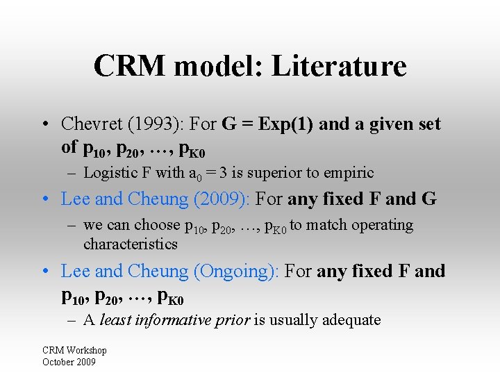
CRM model: Literature • Chevret (1993): For G = Exp(1) and a given set of p 10, p 20, …, p. K 0 – Logistic F with a 0 = 3 is superior to empiric • Lee and Cheung (2009): For any fixed F and G – we can choose p 10, p 20, …, p. K 0 to match operating characteristics • Lee and Cheung (Ongoing): For any fixed F and p 10, p 20, …, p. K 0 – A least informative prior is usually adequate CRM Workshop October 2009

Choice of p 0 k’s (Lee and Cheung, 2009)

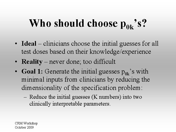
Who should choose p 0 k’s? • Ideal – clinicians choose the initial guesses for all test doses based on their knowledge/experience • Reality – never done; too difficult • Goal 1: Generate the initial guesses p 0 k’s with minimal inputs from clinicians by reducing the dimensionality of the specification problem: – Reduce the initial guesses (K numbers) into two clinically interpretable parameters. CRM Workshop October 2009

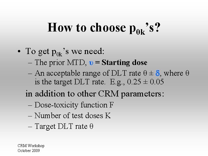
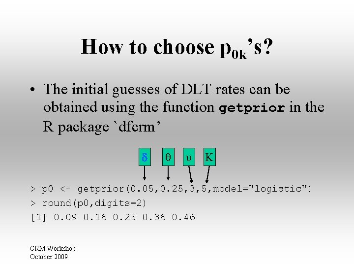
How to choose p 0 k’s? • To get p 0 k’s we need: – The prior MTD, υ = Starting dose – An acceptable range of DLT rate θ ± , where θ is the target DLT rate. E. g. , 0. 25 ± 0. 05 in addition to other CRM parameters: – Dose-toxicity function F – Number of test doses K – Target DLT rate θ CRM Workshop October 2009

How to choose p 0 k’s? • The initial guesses of DLT rates can be obtained using the function getprior in the R package `dfcrm’ θ υ K > p 0 <- getprior(0. 05, 0. 25, 3, 5, model="logistic") > round(p 0, digits=2) [1] 0. 09 0. 16 0. 25 0. 36 0. 46 CRM Workshop October 2009

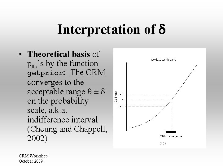
Interpretation of • Theoretical basis of p 0 k’s by the function getprior: The CRM converges to the acceptable range θ ± on the probability scale, a. k. a. indifference interval (Cheung and Chappell, 2002) CRM Workshop October 2009

How to choose ? • Goal 2: Choose empirically (if the clinicians don’t call it) – Asymptotically, a small has a small bias. – With small-moderate sample size, a small has a large variance of selected MTD. – Use simulations to obtain a that yields competitive operating characteristics over a wide range of scenarios CRM Workshop October 2009

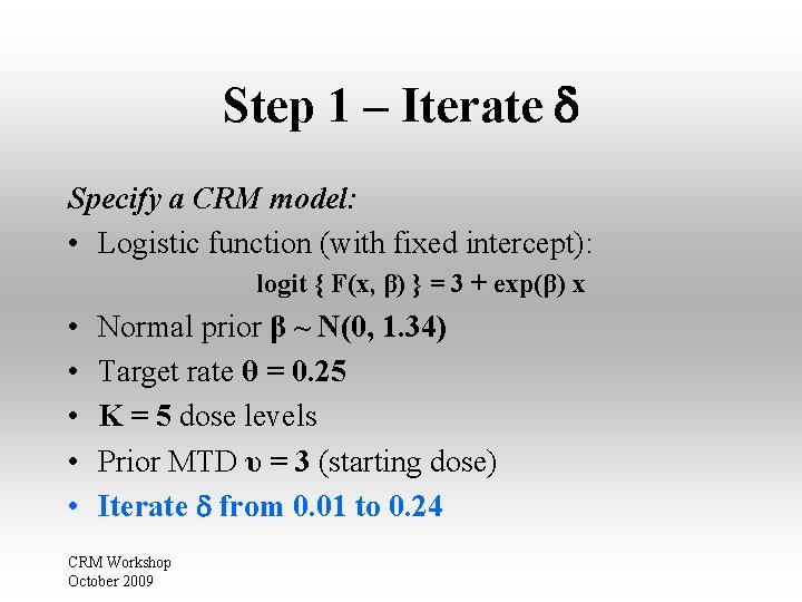
Step 1 – Iterate Specify a CRM model: • Logistic function (with fixed intercept): logit { F(x, β) } = 3 + exp(β) x • • • Normal prior β ~ N(0, 1. 34) Target rate θ = 0. 25 K = 5 dose levels Prior MTD υ = 3 (starting dose) Iterate from 0. 01 to 0. 24 CRM Workshop October 2009

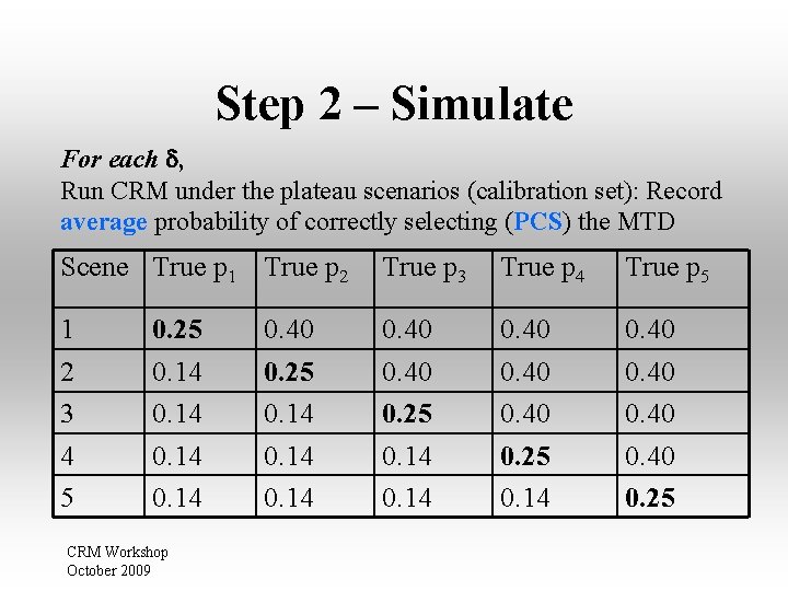
Step 2 – Simulate For each , Run CRM under the plateau scenarios (calibration set): Record average probability of correctly selecting (PCS) the MTD Scene True p 1 True p 2 True p 3 True p 4 True p 5 1 2 3 4 5 0. 40 0. 25 0. 14 0. 40 0. 25 0. 14 CRM Workshop October 2009 0. 40 0. 25 0. 14

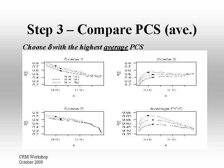
Step 3 – Compare PCS (ave. ) Choose with the highest average PCS CRM Workshop October 2009

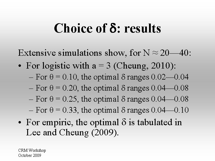
Choice of : results Extensive simulations show, for N ≈ 20— 40: • For logistic with a = 3 (Cheung, 2010): – For θ = 0. 10, the optimal ranges 0. 02— 0. 04 – For θ = 0. 20, the optimal ranges 0. 04— 0. 08 – For θ = 0. 25, the optimal ranges 0. 04— 0. 08 – For θ = 0. 33, the optimal ranges 0. 04— 0. 10 • For empiric, the optimal is tabulated in Lee and Cheung (2009). CRM Workshop October 2009

Choice of prior G(β)

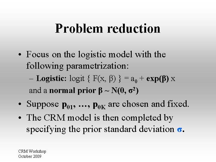
Problem reduction • Focus on the logistic model with the following parametrization: – Logistic: logit { F(x, β) } = a 0 + exp(β) x and a normal prior β ~ N(0, σ2) • Suppose p 01, …, p 0 K are chosen and fixed. • The CRM model is then completed by specifying the prior standard deviation σ. CRM Workshop October 2009

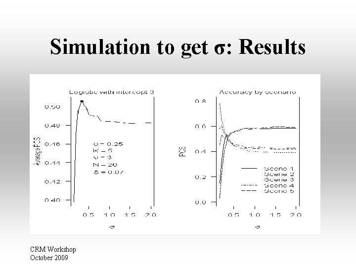
Simulation to get σ • 1 st try: Use the same simulation approach as before: 1. Iterate σ: Fix all CRM parameters but σ 2. Simulate: Run CRM under the plateau scenarios 3. Compare PCS: Choose σ with the highest average PCS CRM Workshop October 2009

Simulation to get σ: Results CRM Workshop October 2009

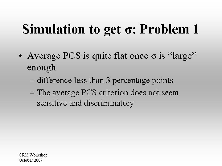
Simulation to get σ: Problem 1 • Average PCS is quite flat once σ is “large” enough – difference less than 3 percentage points – The average PCS criterion does not seem sensitive and discriminatory CRM Workshop October 2009

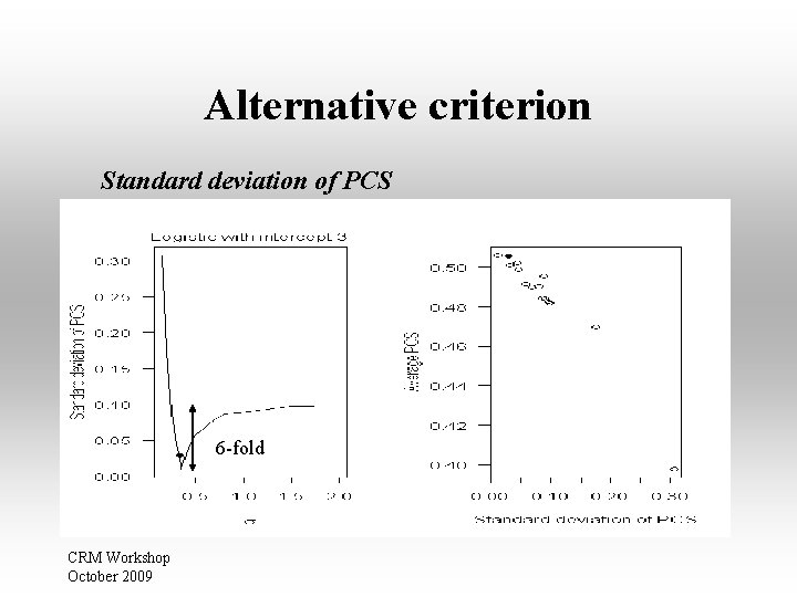
Alternative criterion Standard deviation of PCS 6 -fold CRM Workshop October 2009

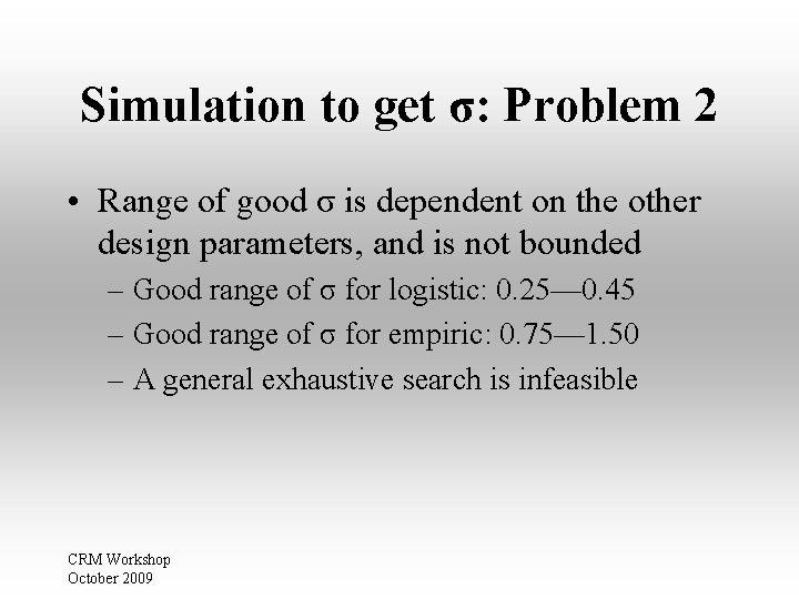
Simulation to get σ: Problem 2 • Range of good σ is dependent on the other design parameters, and is not bounded – Good range of σ for logistic: 0. 25— 0. 45 – Good range of σ for empiric: 0. 75— 1. 50 – A general exhaustive search is infeasible CRM Workshop October 2009

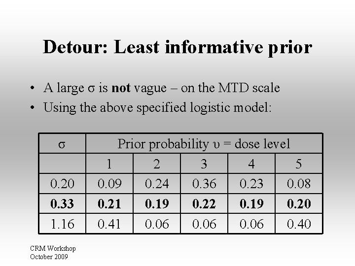
Detour: Least informative prior • A large σ is not vague – on the MTD scale • Using the above specified logistic model: σ 0. 20 0. 33 1. 16 CRM Workshop October 2009 Prior probability υ = dose level 1 2 3 4 5 0. 09 0. 24 0. 36 0. 23 0. 08 0. 21 0. 19 0. 22 0. 19 0. 20 0. 41 0. 06 0. 40

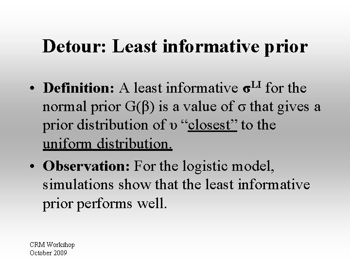
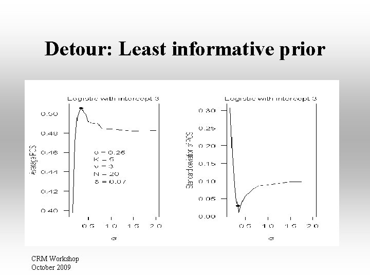
Detour: Least informative prior • Definition: A least informative σLI for the normal prior G(β) is a value of σ that gives a prior distribution of υ “closest” to the uniform distribution. • Observation: For the logistic model, simulations show that the least informative prior performs well. CRM Workshop October 2009

Detour: Least informative prior CRM Workshop October 2009

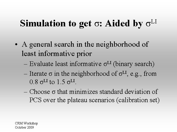
Simulation to get σ: Aided by σLI • A general search in the neighborhood of least informative prior – Evaluate least informative σLI (binary search) – Iterate σ in the neighborhood of σLI, e. g. , from 0. 8 σLI to 1. 5 σLI. – Choose σ that minimizes standard deviation of PCS over the plateau scenarios (calibration set) CRM Workshop October 2009

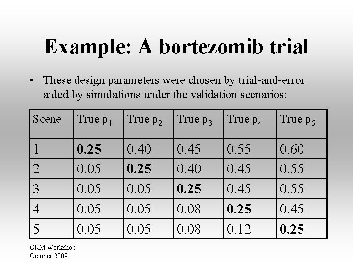
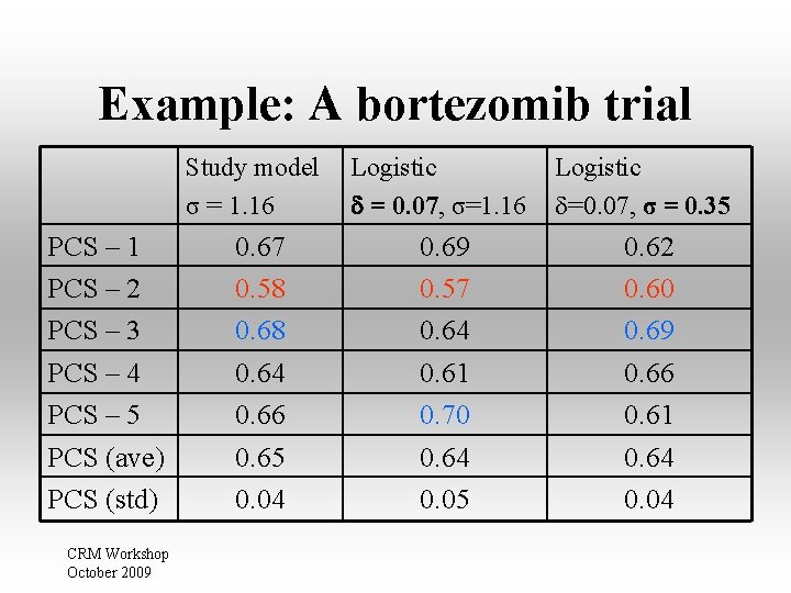
Example: A bortezomib trial • Leonard, Furman, Cheung, et al. (2006): CHOP-R + escalation dose of bortezomib in lymphoma patients • Trial design: (TITE-)CRM with – θ = 0. 25, K = 5, υ = 3 – p 01=. 05, p 02=. 12, p 03=. 25, p 04=. 40, p 05=. 55 – Empiric F(x, β) = xexp(β) – β ~ N(0, 1. 34) CRM Workshop October 2009

Example: A bortezomib trial • These design parameters were chosen by trial-and-error aided by simulations under the validation scenarios: Scene True p 1 True p 2 True p 3 True p 4 True p 5 1 2 3 4 5 0. 25 0. 05 0. 40 0. 25 0. 08 0. 55 0. 45 0. 25 0. 12 0. 60 0. 55 0. 45 0. 25 CRM Workshop October 2009

Example: A bortezomib trial PCS – 1 PCS – 2 PCS – 3 PCS – 4 PCS – 5 PCS (ave) PCS (std) CRM Workshop October 2009 Study model σ = 1. 16 Logistic = 0. 07, σ=1. 16 Logistic =0. 07, σ = 0. 35 0. 67 0. 58 0. 64 0. 66 0. 65 0. 04 0. 69 0. 57 0. 64 0. 61 0. 70 0. 64 0. 05 0. 62 0. 60 0. 69 0. 66 0. 61 0. 64 0. 04

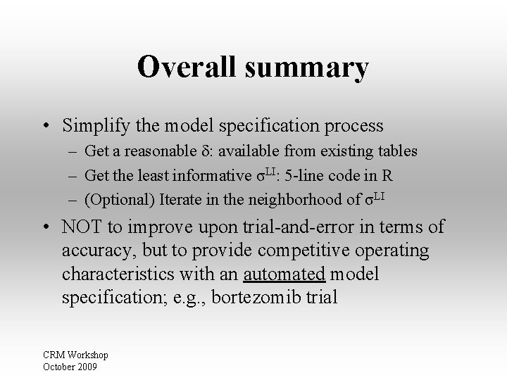
Overall summary • Simplify the model specification process – Get a reasonable : available from existing tables – Get the least informative σLI: 5 -line code in R – (Optional) Iterate in the neighborhood of σLI • NOT to improve upon trial-and-error in terms of accuracy, but to provide competitive operating characteristics with an automated model specification; e. g. , bortezomib trial CRM Workshop October 2009

Resources • `dfcrm’ package in R – http: //www. r-project. org • Lee and Cheung (2009): Model calibration in the continual reassessment method. Clinical Trials 6: 227— 238. • Ongoing: Tabulate the values of ( , σ) for a wide range of (θ, K, υ, N). CRM Workshop October 2009