Species diversity Concept of diversity Informally variety Wallaces

Species diversity

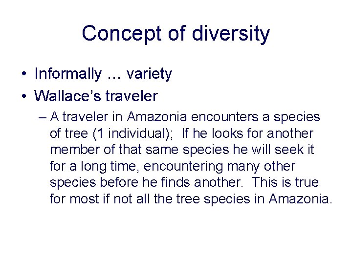
Concept of diversity • Informally … variety • Wallace’s traveler – A traveler in Amazonia encounters a species of tree (1 individual); If he looks for another member of that same species he will seek it for a long time, encountering many other species before he finds another. This is true for most if not all the tree species in Amazonia.

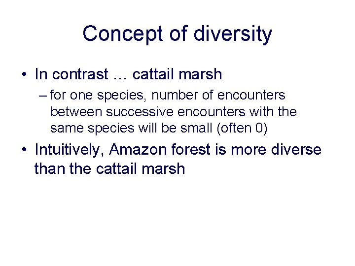
Concept of diversity • In contrast … cattail marsh – for one species, number of encounters between successive encounters with the same species will be small (often 0) • Intuitively, Amazon forest is more diverse than the cattail marsh

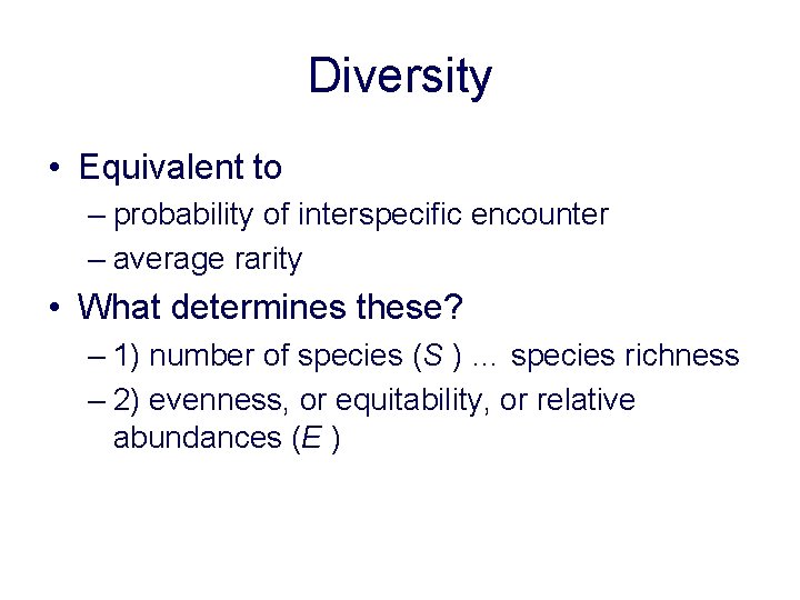
Diversity • Equivalent to – probability of interspecific encounter – average rarity • What determines these? – 1) number of species (S ) … species richness – 2) evenness, or equitability, or relative abundances (E )

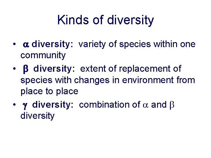
Kinds of diversity • a diversity: variety of species within one community • b diversity: extent of replacement of species with changes in environment from place to place • g diversity: combination of a and b diversity

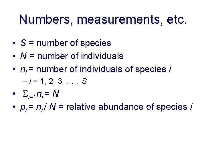
Numbers, measurements, etc. • S = number of species • N = number of individuals • ni = number of individuals of species i – i = 1, 2, 3, … , S • Si=1 ni = N • pi = ni / N = relative abundance of species i

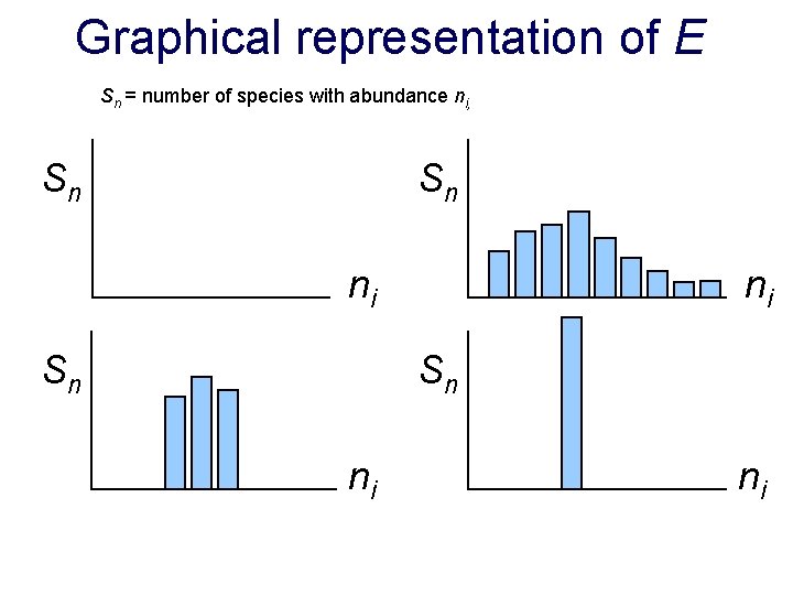
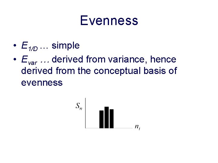
Graphical representation of E Sn = number of species with abundance ni, Sn Sn ni ni

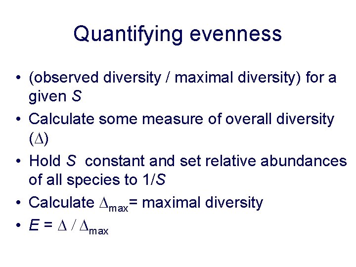
Quantifying evenness • (observed diversity / maximal diversity) for a given S • Calculate some measure of overall diversity (D) • Hold S constant and set relative abundances of all species to 1/S • Calculate Dmax= maximal diversity • E = D / Dmax

Diversity indices • Single number combining species number and evenness • >60 different formulas • differ in relative weight given to evenness or species number

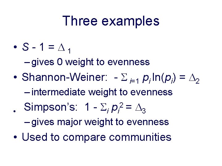
Three examples • S-1=D 1 – gives 0 weight to evenness • Shannon-Weiner: - S i=1 pi ln(pi) = D 2 – intermediate weight to evenness • Simpson’s: 1 - Si pi 2 = D 3 – gives major weight to evenness • Used to compare communities

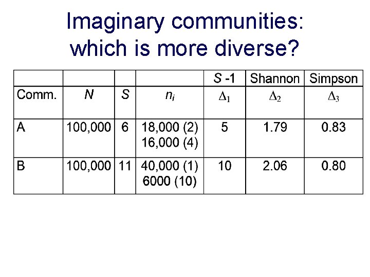
Imaginary communities: which is more diverse?

Different comparisons • Indices do not measure a single quantity • Diversity indices combine 2 inherently different quantities • Weights chosen are arbitrary • Indices are related in a complex way

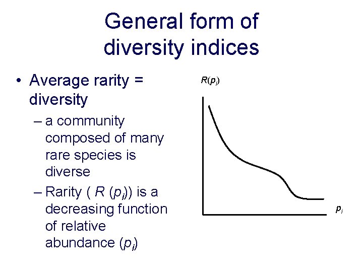
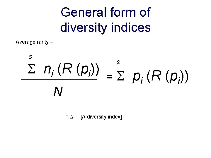
General form of diversity indices • Average rarity = diversity – a community composed of many rare species is diverse – Rarity ( R (pi)) is a decreasing function of relative abundance (pi) R(pi) pi

General form of diversity indices Average rarity = S S ni (R (pi)) S =S N =D [A diversity index] pi (R (pi))

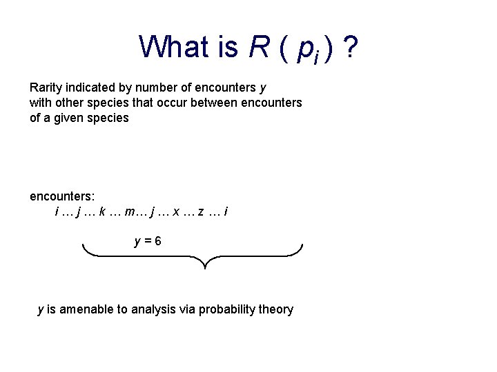
What is R ( pi ) ? Rarity indicated by number of encounters y with other species that occur between encounters of a given species encounters: i … j … k … m… j … x … z … i y=6 y is amenable to analysis via probability theory

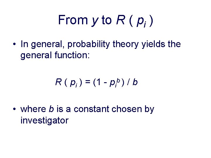
From y to R ( pi ) • In general, probability theory yields the general function: R ( pi ) = (1 - pib ) / b • where b is a constant chosen by investigator

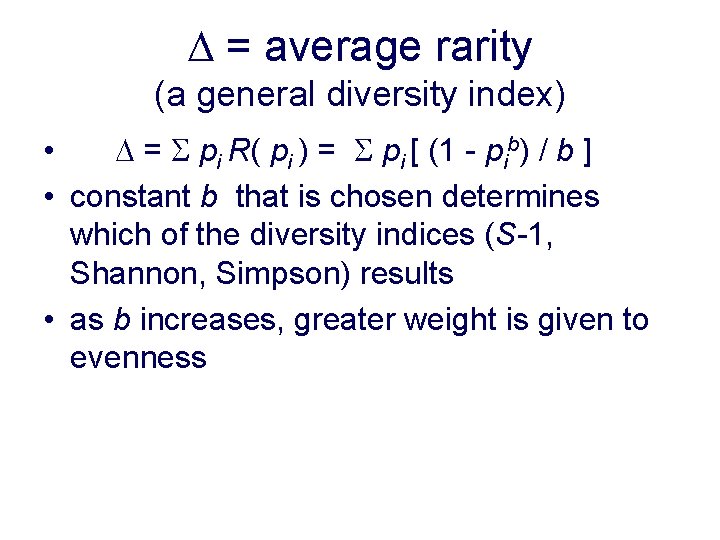
D = average rarity (a general diversity index) • D = S pi R( pi ) = S pi [ (1 - pib) / b ] • constant b that is chosen determines which of the diversity indices (S-1, Shannon, Simpson) results • as b increases, greater weight is given to evenness

Three diversity indices

Diversity indices • Shows that they are related • Differ in R( pi ) • Does not solve the problem… which weighting is correct • Solution: don’t bother with diversity indices • implies that diversity as a single thing doesn’t exist

Quantifying diversity • Report S – in a sample S depends on N – to compare samples of different sizes use rarefaction • Report E – many measures depend on S – choose those least dependent on S

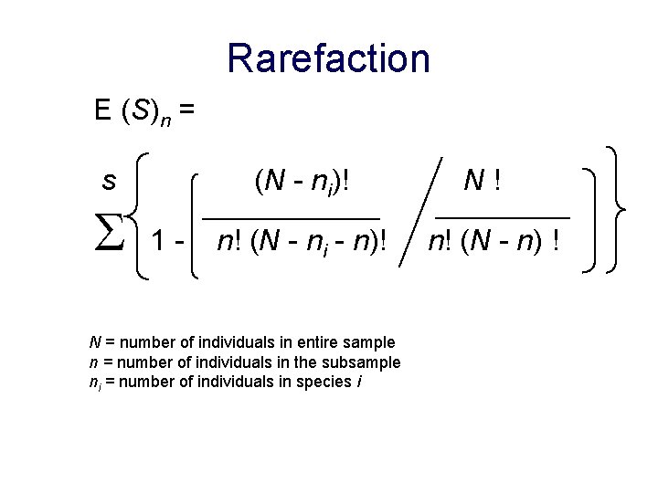
Rarefaction • two samples of different N • lower N, lower S in the sample, regardless of S in the community itself • Rarefaction … estimating expected number of species in a sample of size n : • E (S )n

Rarefaction E (S)n = s S (N - ni)! 1 - n! (N - ni - n)! N = number of individuals in entire sample n = number of individuals in the subsample ni = number of individuals in species i N! n! (N - n) !

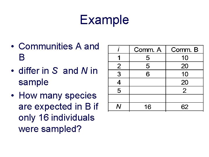
Example • Communities A and B • differ in S and N in sample • How many species are expected in B if only 16 individuals were sampled?

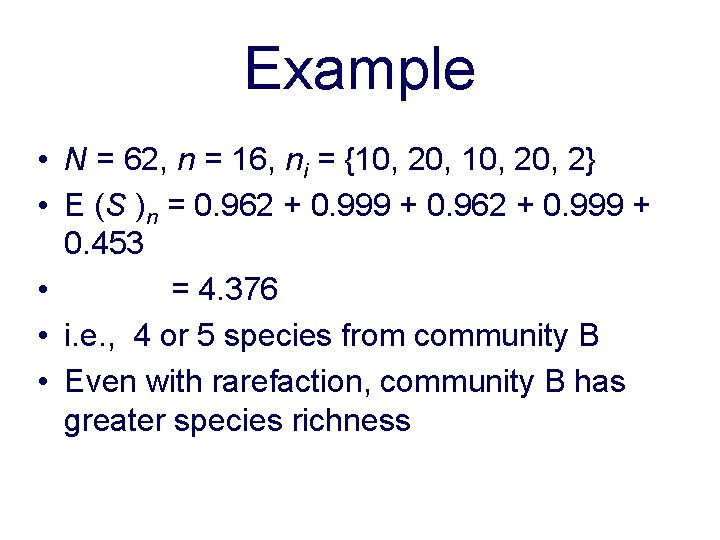
Example • N = 62, n = 16, ni = {10, 20, 2} • E (S )n = 0. 962 + 0. 999 + 0. 453 • = 4. 376 • i. e. , 4 or 5 species from community B • Even with rarefaction, community B has greater species richness

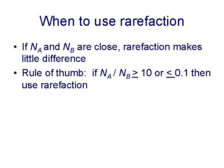
When to use rarefaction • If NA and NB are close, rarefaction makes little difference • Rule of thumb: if NA / NB > 10 or < 0. 1 then use rarefaction

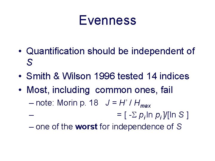
Evenness • Quantification should be independent of S • Smith & Wilson 1996 tested 14 indices • Most, including common ones, fail – note: Morin p. 18 J = H’ / Hmax – = [ -S pi ln pi ]/[ln S ] – one of the worst for independence of S

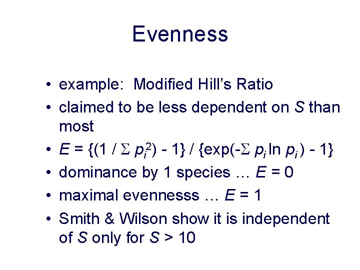
Evenness • example: Modified Hill’s Ratio • claimed to be less dependent on S than most • E = {(1 / S pi 2) - 1} / {exp(-S pi ln pi ) - 1} • dominance by 1 species … E = 0 • maximal evennesss … E = 1 • Smith & Wilson show it is independent of S only for S > 10

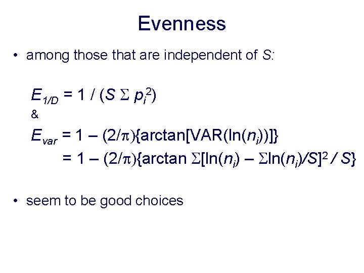
Evenness • among those that are independent of S: E 1/D = 1 / (S S pi 2) & Evar = 1 – (2/p){arctan[VAR(ln(ni))]} = 1 – (2/p){arctan S[ln(ni) – Sln(ni)/S]2 / S} • seem to be good choices

Evenness • E 1/D … simple • Evar … derived from variance, hence derived from the conceptual basis of evenness

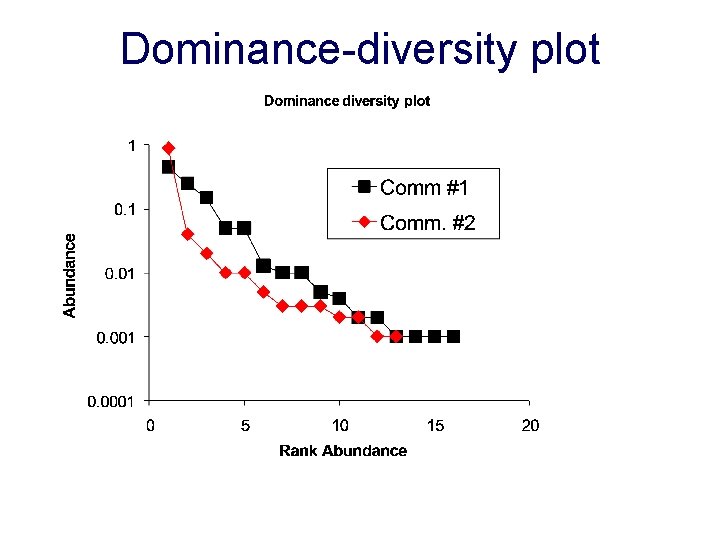
Dominance-diversity plot

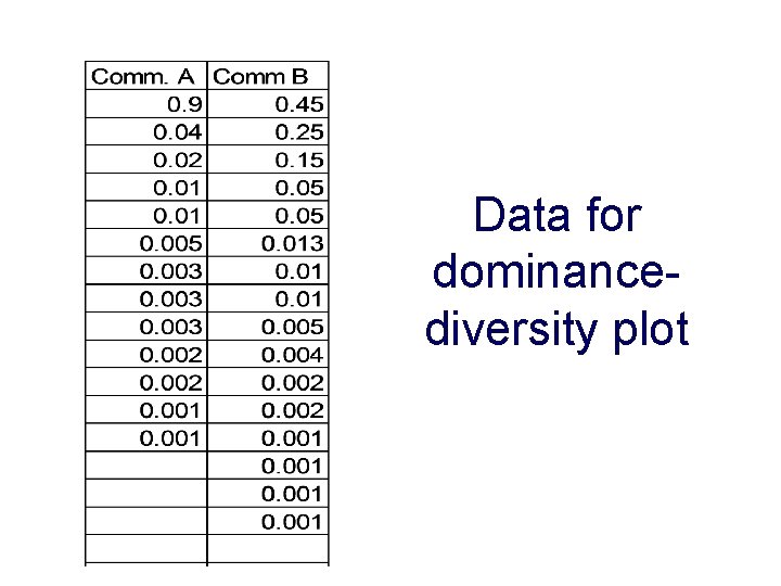
Data for dominancediversity plot

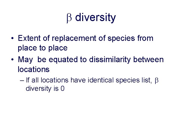
b diversity • Extent of replacement of species from place to place • May be equated to dissimilarity between locations – If all locations have identical species list, b diversity is 0

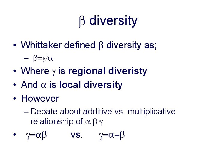
b diversity • Whittaker defined b diversity as; – b=g/a • Where g is regional diveristy • And a is local diversity • However – Debate about additive vs. multiplicative relationship of a b g • g=ab vs. g=a+b

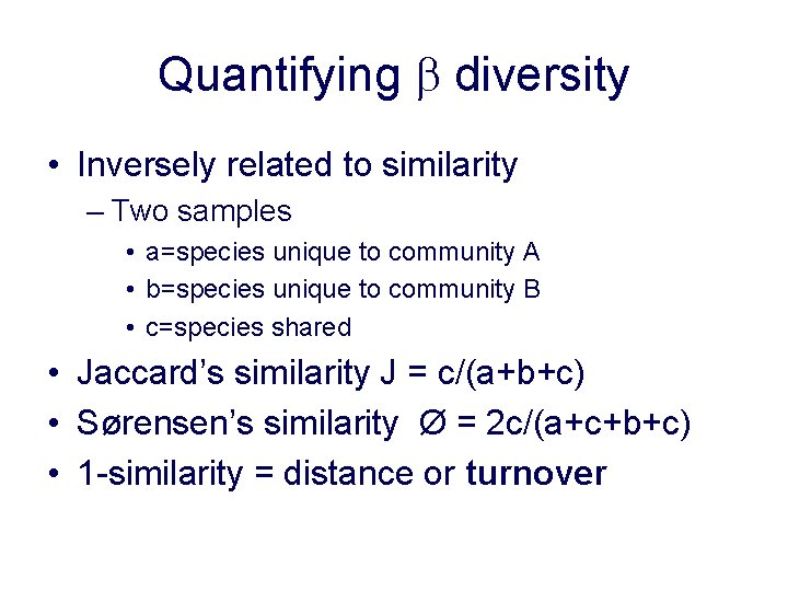
Quantifying b diversity • Inversely related to similarity – Two samples • a=species unique to community A • b=species unique to community B • c=species shared • Jaccard’s similarity J = c/(a+b+c) • Sørensen’s similarity Ø = 2 c/(a+c+b+c) • 1 -similarity = distance or turnover

Quantifying b diversity • Whittaker’s index – b = (a+b+c)/{[a+c+b+c]/2} – 1 – = (Stotal / S) -1 • Works with >2 samples. • NOTE: none of these weight species by abundances – (i. e. , none incorporate evenness)

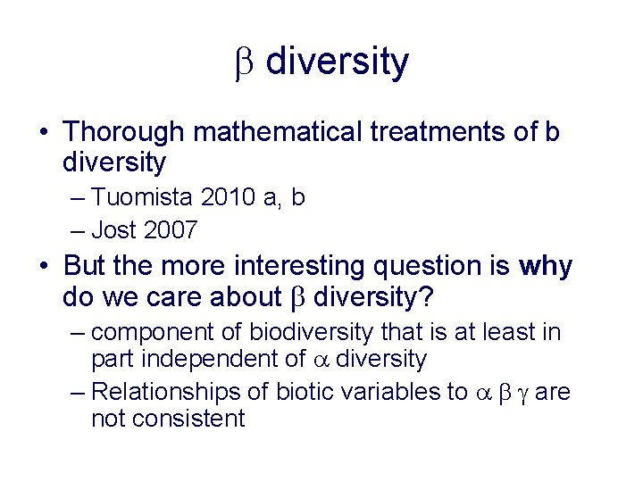
b diversity • Thorough mathematical treatments of b diversity – Tuomista 2010 a, b – Jost 2007 • But the more interesting question is why do we care about b diversity? – component of biodiversity that is at least in part independent of a diversity – Relationships of biotic variables to a b g are not consistent

Diversity Productivity Stability

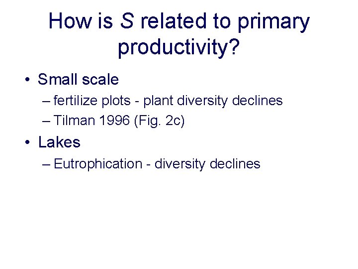
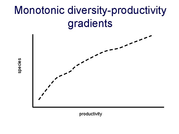
How is S related to primary productivity? • Small scale – fertilize plots - plant diversity declines – Tilman 1996 (Fig. 2 c) • Lakes – Eutrophication - diversity declines

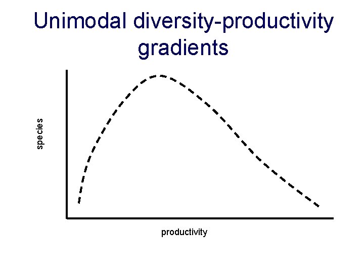
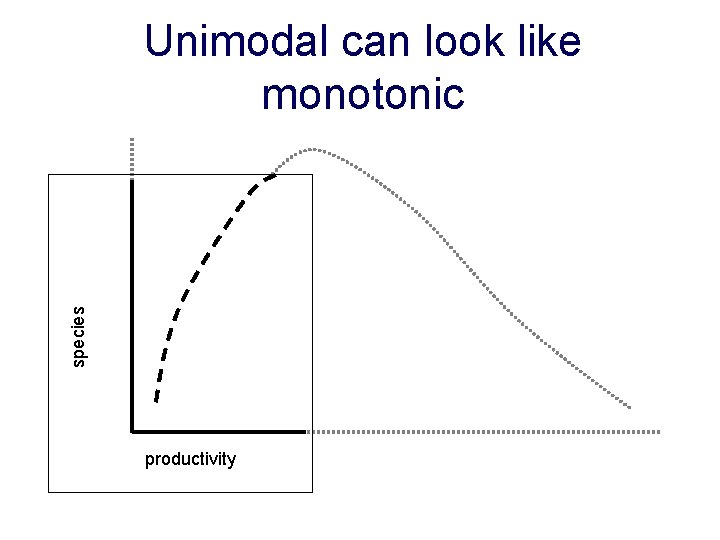
species Unimodal diversity-productivity gradients productivity

species Monotonic diversity-productivity gradients productivity

species Unimodal can look like monotonic productivity

Why should diversity decline with productivity? • High productivity reduced spatial heterogeneity in resources • Spatial heterogeneity fosters diversity – reduces competitive exclusion – variance in resource ratio hypothesis (VRR) – each species does best on a particular ratio of resources – e. g. , plants and soil nutrients

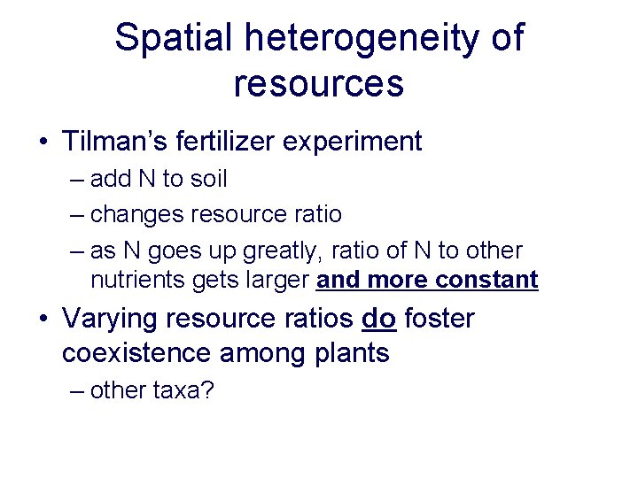
Spatial heterogeneity of resources • Tilman’s fertilizer experiment – add N to soil – changes resource ratio – as N goes up greatly, ratio of N to other nutrients gets larger and more constant • Varying resource ratios do foster coexistence among plants – other taxa?

VRR Hypothesis • Assumes – species occur in patches – competition is local – resource competition • Generality? – Rodents? – Benthic invertebrates? – Tropical mammals?

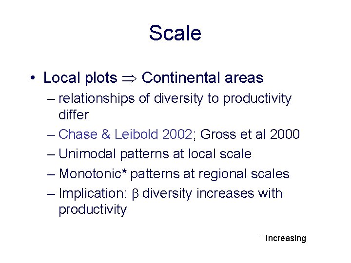
Scale • Local plots Continental areas – relationships of diversity to productivity differ – Chase & Leibold 2002; Gross et al 2000 – Unimodal patterns at local scale – Monotonic* patterns at regional scales – Implication: b diversity increases with productivity * Increasing

Scale • Same mechanism at all scales? – VRR works best at local plot scale – Applicability at larger scales unknown – Does natural variation in productivity affect species the same way as experimental manipulation?

Alternative interpretations (Abrams 1995) • Challenges interpretation of monotonic patterns as artefacts of inadequate sampling • Questions the assumption that unimodal patterns must be due to competition – need for experimental data on competition – experimental test of VRR • Alternative hypotheses predict monotonic relationships

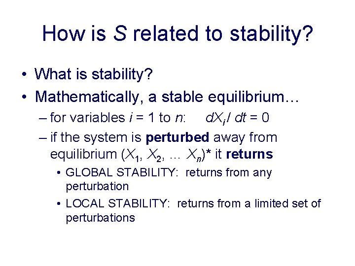
How is S related to stability? • What is stability? • Mathematically, a stable equilibrium… – for variables i = 1 to n: d. Xi / dt = 0 – if the system is perturbed away from equilibrium (X 1, X 2, … Xn)* it returns • GLOBAL STABILITY: returns from any perturbation • LOCAL STABILITY: returns from a limited set of perturbations

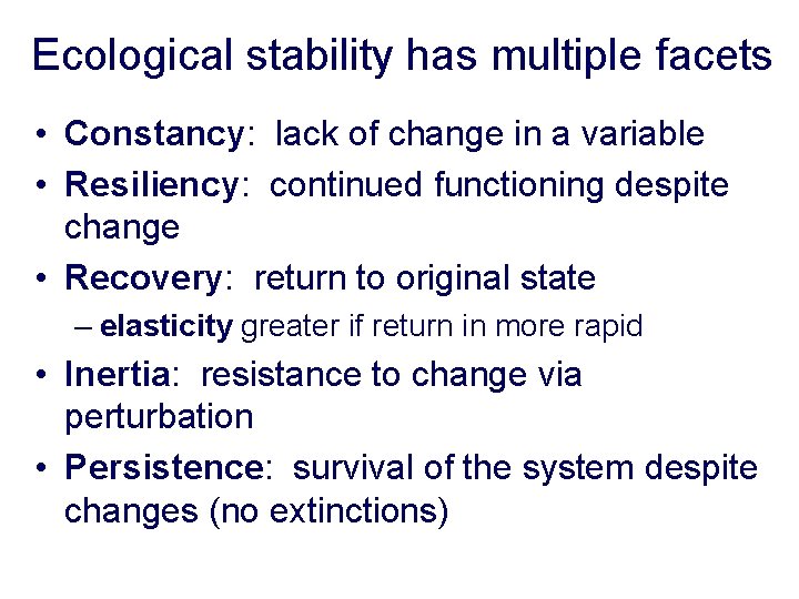
Ecological stability has multiple facets • Constancy: lack of change in a variable • Resiliency: continued functioning despite change • Recovery: return to original state – elasticity greater if return in more rapid • Inertia: resistance to change via perturbation • Persistence: survival of the system despite changes (no extinctions)

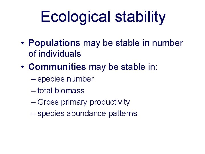
Ecological stability • Populations may be stable in number of individuals • Communities may be stable in: – species number – total biomass – Gross primary productivity – species abundance patterns

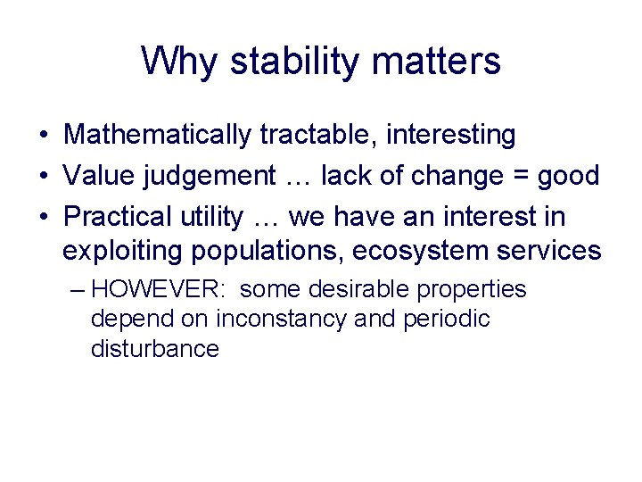
Why stability matters • Mathematically tractable, interesting • Value judgement … lack of change = good • Practical utility … we have an interest in exploiting populations, ecosystem services – HOWEVER: some desirable properties depend on inconstancy and periodic disturbance

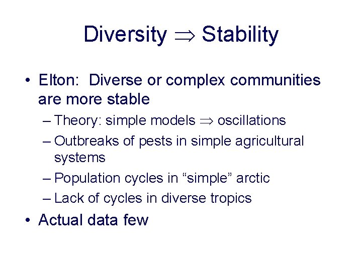
Diversity Stability • Elton: Diverse or complex communities are more stable – Theory: simple models oscillations – Outbreaks of pests in simple agricultural systems – Population cycles in “simple” arctic – Lack of cycles in diverse tropics • Actual data few

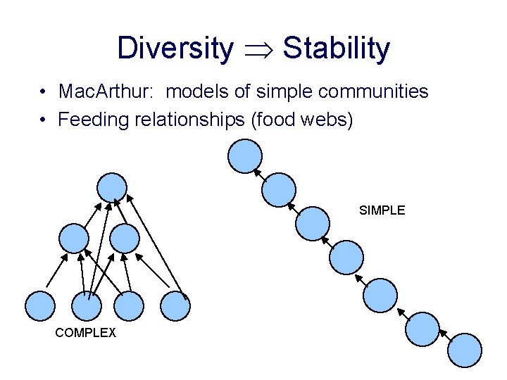
Diversity Stability • Mac. Arthur: models of simple communities • Feeding relationships (food webs) SIMPLE COMPLEX

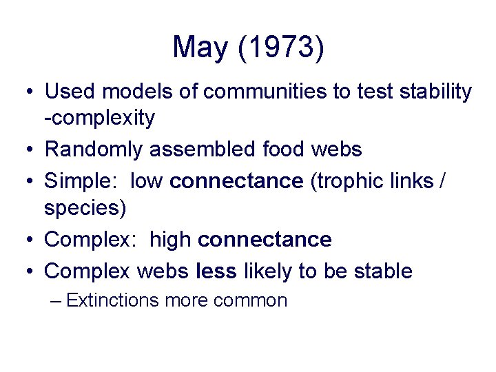
May (1973) • Used models of communities to test stability -complexity • Randomly assembled food webs • Simple: low connectance (trophic links / species) • Complex: high connectance • Complex webs less likely to be stable – Extinctions more common

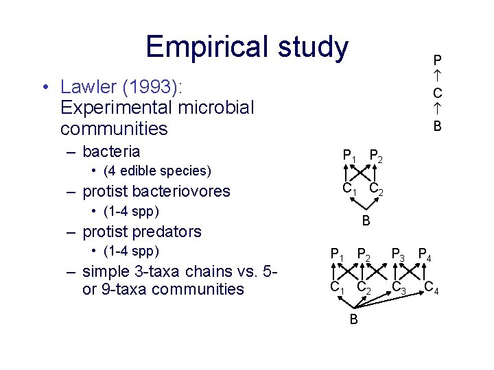
Empirical study P C B • Lawler (1993): Experimental microbial communities – bacteria • (4 edible species) – protist bacteriovores P 1 P 2 C 1 C 2 • (1 -4 spp) B – protist predators • (1 -4 spp) – simple 3 -taxa chains vs. 5 or 9 -taxa communities P 1 P 2 P 3 P 4 C 1 C 2 C 3 B C 4

Lawler 1993 • Extinctions – 9 -taxa > 5 -taxa > 3 -taxa communities – consistent with May’s model results – diversity (or complexity) leads to instability – but population variation was not greater with greater diversity (for most of the species)

How did ecologists conclude complexity stability? • Elton – particularly concerned about human impact – simplification systems – need to preserve natural systems • Complexity and stability both valued • Assumed observed natural systems were stable (return to equilibrium)

Any resolution? • Complexity inconstancy – numbers of species change readily • Complexity resiliency – function despite change • Stability & complexity (or diversity) may be related, but not simply – abiotic stability or predictability may foster evolution of complexity

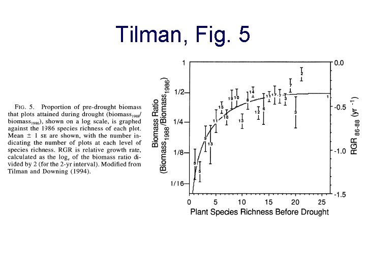
Tilman 1996 • Experimental manipulation of productivity – Soil N – Produces a range of diversities (S ) in plots • Diversity and productivity are related – How do plots respond to natural perturbations? • annual variation, particularly drought (1988) • Three measures of biomass – change in biomass pre-drought - peak drought – CV biomass over 10 years – CV biomass in non-drought years

Whole community response: Total biomass • All measures indicate greater stability with greater S – change in biomass lower with greater S – CV’s less with greater S • Mc. Naughton obtained similar results with respect to grazing as a disturbance

Tilman, Fig. 5

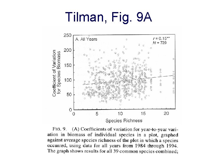
Individual species responses: Biomass • Averaged across species (39) • Lower stability of populations with greater S – CV’s greater with greater S – both drought and non-drought years • Population stability (average) decreases with diversity

Tilman, Fig. 9 A