Specialized Custom DOE for Experienced Experimenters Tom Donnelly

Specialized Custom DOE for Experienced Experimenters Tom Donnelly JMP Systems Engineer Tom. Donnelly@jmp. com Copyright © SAS Inst itute Inc. All rig hts reserved.

Agenda Multiple Response Optimization – Trade-Space Analysis • Review of Classic DOE • Real-World Experimental Issues – Custom DOE is about Making • Designs Fit the Problem – NOT Making Problems Fit the Designs • Three Example Designs • Augment a broken design with constraints • Augment a screening design to RSM (sequential experimentation) • Create a design from a candidate set of trials – a good way to examine historical (haphazard) data Copyright © SAS Inst itute Inc. All rig hts reserved.

Why use DOE? Quicker answers, lower costs, solve bigger problems More rapidly answer “what if? ” questions • Do sensitivity and trade-space analysis • Optimize across multiple responses • By running efficient subsets of all possible combinations, one can – for the same resources and constraints – solve bigger • problems • By running sequences of designs one can be as cost effective as possible and run no more trials than needed to get a useful answer Copyright © SAS Inst itute Inc. All rig hts reserved.

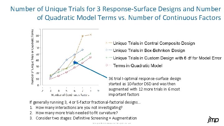
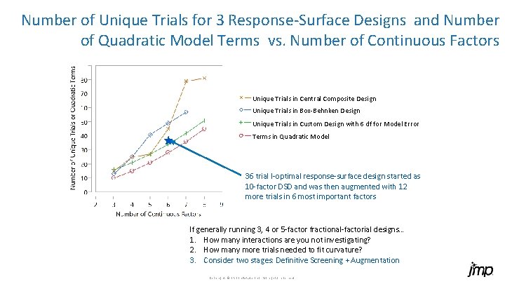
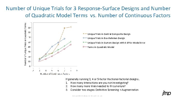
Number of Unique Trials for 3 Response-Surface Designs and Number of Quadratic Model Terms vs. Number of Continuous Factors 36 trial I-optimal response-surface design started as 10 -factor DSD and was then augmented with 12 more trials in 6 most important factors If generally running 3, 4 or 5 -factor fractional-factorial designs… 1. How many interactions are you not investigating? 2. How many more trials needed to fit curvature? 3. Consider two stages: Definitive Screening + Augmentation Copyright © SAS Inst itute Inc. All rig hts reserved.

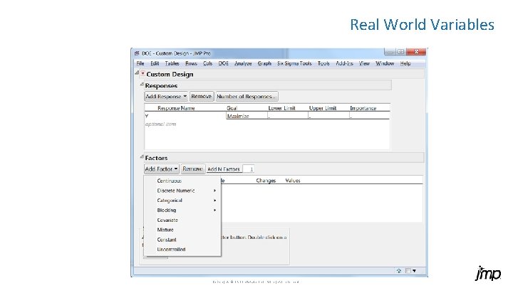
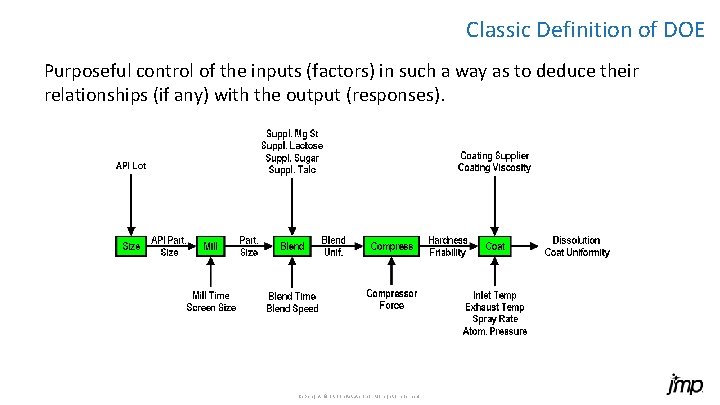
Real-World Design Issues How many experimenters have any of these issues? Most of these are NOT well treated by classic DOE. Work with these different kinds of control variables/factors: • • Continuous/quantitative? Finely adjustable like temperature, speed, force • Categorical/qualitative? Comes in types, like material = rubber, polycarbonate, steel with mixed # of levels; 3 chemical agents, 4 decontaminants, 8 coupon materials… • Mixture/formulation? Blend different amounts of ingredients and the process performance is dependent on the proportions more than on the amounts • Blocking? e. g. “lots” of the same raw materials, multiple “same” machines, samples get processed in “groups” – like “eight in a tray, ” run tests over multiple days – i. e. variables for which there shouldn’t be a causal effect Work with combinations of these four kinds of variables? • Certain combinations cannot be run? (too costly, unsafe, breaks the process) • Would like to add onto existing trials? (really expensive/time consuming to run) • My design broke! Repair design by augmenting with constraints. • Copyright © SAS Inst itute Inc. All rig hts reserved.

Real World Variables Copyright © SAS Inst itute Inc. All rig hts reserved.

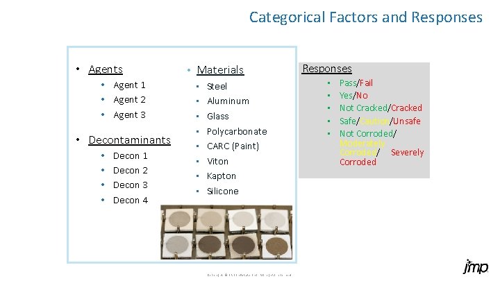
Categorical Factors and Responses • Agent 1 • Agent 2 • Agent 3 • Decontaminants • • Decon 1 Decon 2 Decon 3 Decon 4 • Materials • • Steel Aluminum Glass Polycarbonate CARC (Paint) Viton Kapton Silicone Copyright © SAS Inst itute Inc. All rig hts reserved. Responses • • • Pass/Fail Yes/No Not Cracked/Cracked Safe/Caution/Unsafe Not Corroded/ Moderately Corroded/ Severely Corroded

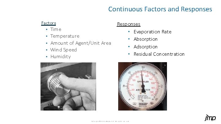
Continuous Factors and Responses Factors • • • Time Temperature Amount of Agent/Unit Area Wind Speed Humidity Responses • Evaporation Rate • Absorption • Adsorption • Residual Concentration Copyright © SAS Inst itute Inc. All rig hts reserved.

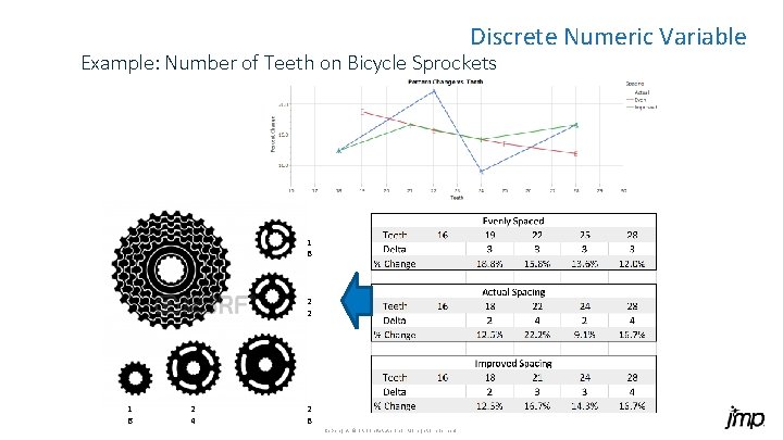
Discrete Numeric Variable Example: Number of Teeth on Bicycle Sprockets 1 8 2 2 1 6 2 4 2 8 Copyright © SAS Inst itute Inc. All rig hts reserved.

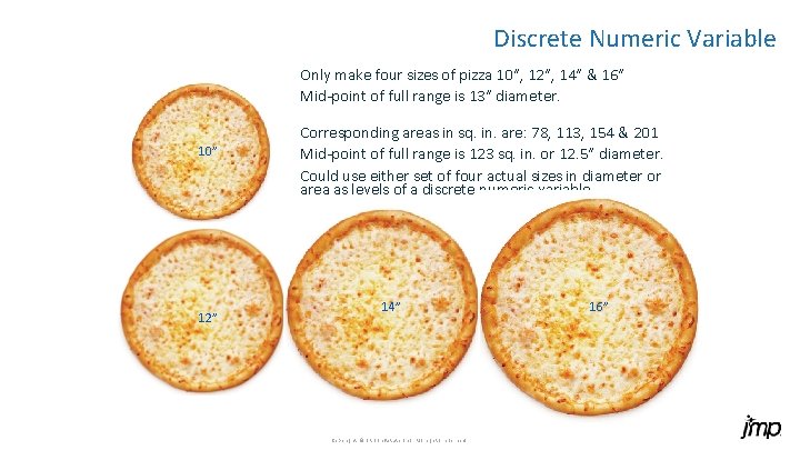
Discrete Numeric Variable Only make four sizes of pizza 10”, 12”, 14” & 16” Mid-point of full range is 13” diameter. 10” 12” Corresponding areas in sq. in. are: 78, 113, 154 & 201 Mid-point of full range is 123 sq. in. or 12. 5” diameter. Could use either set of four actual sizes in diameter or area as levels of a discrete numeric variable. 14” Copyright © SAS Inst itute Inc. All rig hts reserved. 16”

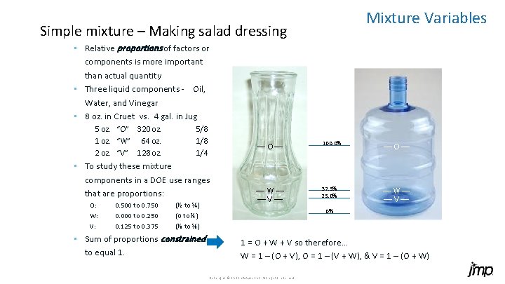
Mixture Variables Simple mixture – Making salad dressing • Relative proportions of factors or components is more important than actual quantity • Three liquid components - Oil, Water, and Vinegar • 8 oz. in Cruet vs. 4 gal. in Jug 5 oz. “O” 320 oz. 1 oz. “W” 64 oz. 2 oz. “V” 128 oz. 5/8 1/4 –– O –– 100. 0% –– O –– –– W –– –– V –– 37. 5% 25. 0% –– W –– –– V –– • To study these mixture components in a DOE use ranges that are proportions: O: W: V: 0. 500 to 0. 750 0. 000 to 0. 250 0. 125 to 0. 375 (½ to ¾) (0 to ¼) (⅛ to ⅜) • Sum of proportions constrained to equal 1. 0% 1 = O + W + V so therefore… W = 1 – (O + V), O = 1 – (V + W), & V = 1 – (O + W) Copyright © SAS Inst itute Inc. All rig hts reserved.

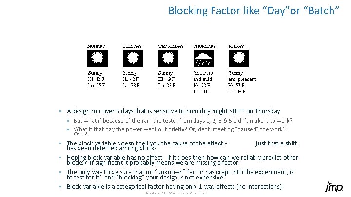
Blocking Factor like “Day”or “Batch” • A design run over 5 days that is sensitive to humidity might SHIFT on Thursday § But what if because of the rain the tester from days 1, 2, 3 & 5 didn’t make it to work? § What if that day the power went out briefly? Or, dept. meeting “paused” the work? Or…? • The block variable doesn’t tell you the cause of the effect - just that a shift has been detected among blocks. • Hoping block variable has no effect. If it does then how can we reliably predict other blocks? If significant it probably means we are missing a factor. • The only way to be sure that no “unknown” factor has crept into the experiment, is to test for it - and “blocking” your design is not expensive. • Block variable is a categorical factor having only 1 -way effects (no interactions) Copyright © SAS Inst itute Inc. All rig hts reserved.

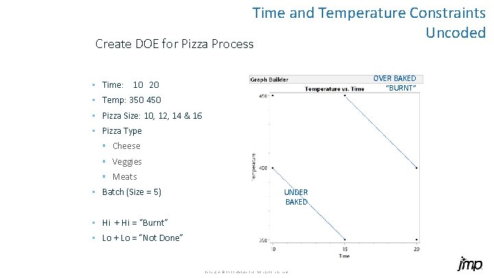
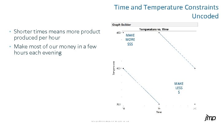
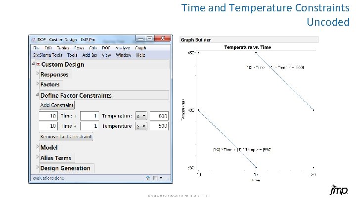
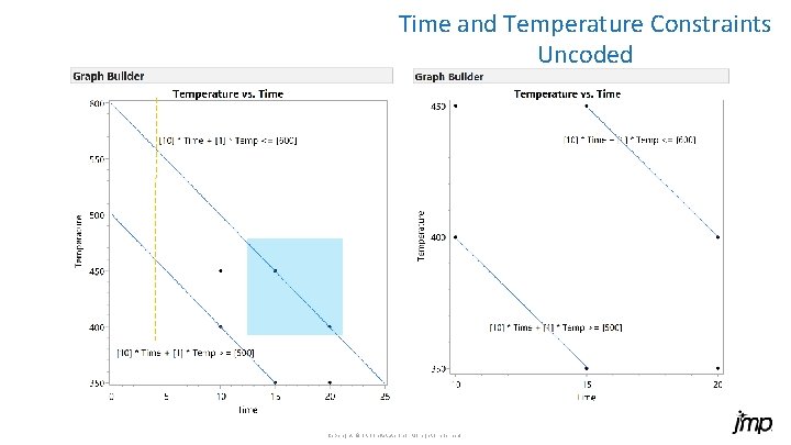
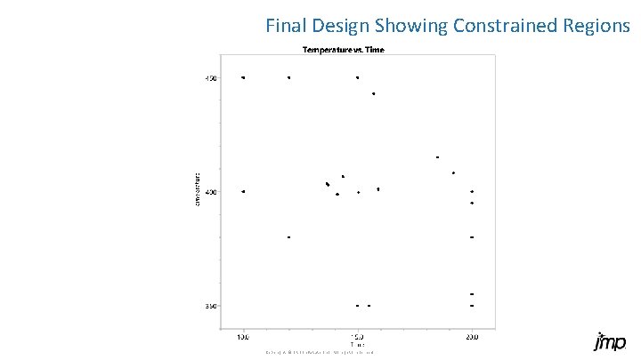
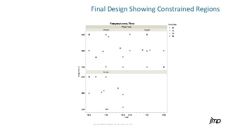
Time and Temperature Constraints Uncoded Create DOE for Pizza Process • Time: OVER BAKED “BURNT” 10 20 • Temp: 350 450 • Pizza Size: 10, 12, 14 & 16 • Pizza Type § Cheese § Veggies § Meats • Batch (Size = 5) UNDER BAKED • Hi + Hi = “Burnt” • Lo + Lo = “Not Done” Copyright © SAS Inst itute Inc. All rig hts reserved.

Time and Temperature Constraints Uncoded Shorter times means more product produced per hour • Make most of our money in a few hours each evening • MAKE MORE $$$ MAKE LESS $ Copyright © SAS Inst itute Inc. All rig hts reserved.

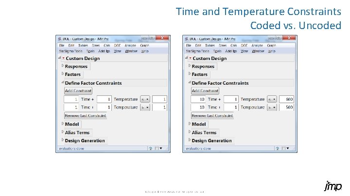
Time and Temperature Constraints Coded vs. Uncoded Copyright © SAS Inst itute Inc. All rig hts reserved.

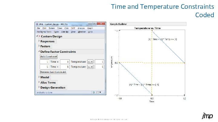
Time and Temperature Constraints Coded Copyright © SAS Inst itute Inc. All rig hts reserved.

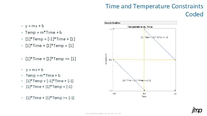
Time and Temperature Constraints Coded y = mx + b • Temp = m*Time + b • [1]*Temp = [-1]*Time + [1] • [1]*Time + [1]*Temp = [1] • • [1]*Time + [1]*Temp <= [1] y = mx + b • Temp = m*Time + b • [1]*Temp = [-1]*Time + [-1] • [1]*Time + [1]*Temp = [-1] • • [1]*Time + [1]*Temp >= [-1] Copyright © SAS Inst itute Inc. All rig hts reserved.

Time and Temperature Constraints Uncoded Copyright © SAS Inst itute Inc. All rig hts reserved.

Time and Temperature Constraints Uncoded Copyright © SAS Inst itute Inc. All rig hts reserved.

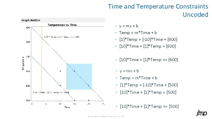
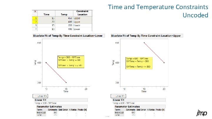
Time and Temperature Constraints Uncoded y = mx + b • Temp = m*Time + b • [1]*Temp = [-10]*Time + [600] • [10]*Time + [1]*Temp = [600] • • [10]*Time + [1]*Temp <= [600] • y = mx + b • Temp = m*Time + b • [1]*Temp = [-10]*Time + [500] • [10]*Time + [1]*Temp = [500] • [10]*Time + [1]*Temp >= [500] Copyright © SAS Inst itute Inc. All rig hts reserved.

Time and Temperature Constraints Uncoded Copyright © SAS Inst itute Inc. All rig hts reserved.

Final Design Showing Constrained Regions Copyright © SAS Inst itute Inc. All rig hts reserved.

Final Design Showing Constrained Regions Copyright © SAS Inst itute Inc. All rig hts reserved.

Definitive Screening Case Study Copyright © SAS Inst itute Inc. All rig hts reserved.

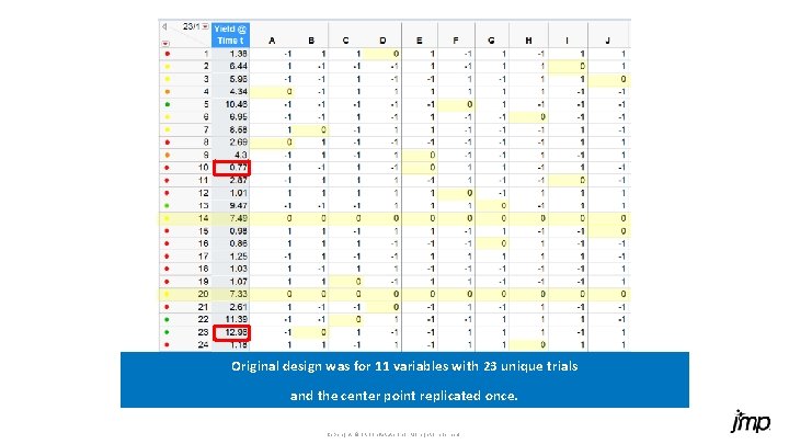
Original design was for 11 variables with 23 unique trials and the center point replicated once. Copyright © SAS Inst itute Inc. All rig hts reserved.

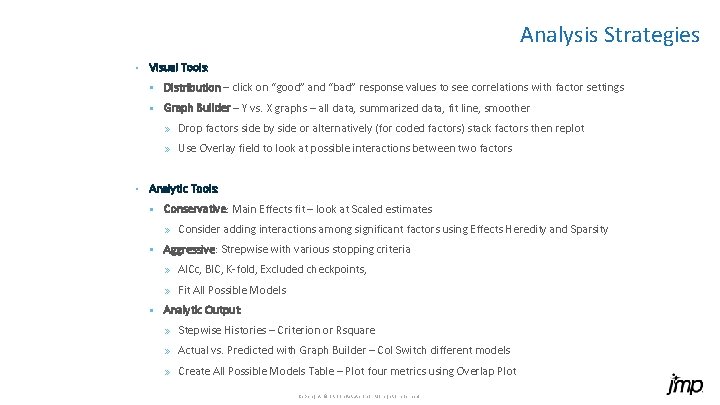
Analysis Strategies • Visual Tools: § Distribution – click on “good” and “bad” response values to see correlations with factor settings § Graph Builder – Y vs. X graphs – all data, summarized data, fit line, smoother » Drop factors side by side or alternatively (for coded factors) stack factors then replot » Use Overlay field to look at possible interactions between two factors • Analytic Tools: § Conservative: Main Effects fit – look at Scaled estimates » Consider adding interactions among significant factors using Effects Heredity and Sparsity § Aggressive: Strepwise with various stopping criteria » AICc, BIC, K-fold, Excluded checkpoints, » Fit All Possible Models § Analytic Output: » Stepwise Histories – Criterion or Rsquare » Actual vs. Predicted with Graph Builder – Col Switch different models » Create All Possible Models Table – Plot four metrics using Overlap Plot Copyright © SAS Inst itute Inc. All rig hts reserved.

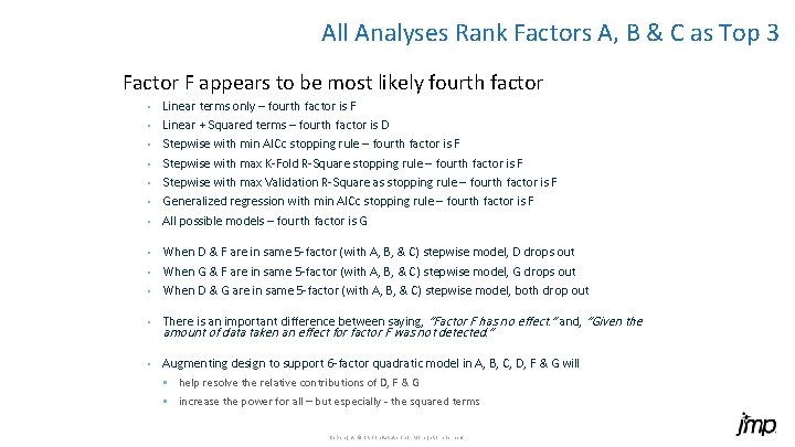
All Analyses Rank Factors A, B & C as Top 3 Factor F appears to be most likely fourth factor • • Linear terms only – fourth factor is F Linear + Squared terms – fourth factor is D Stepwise with min AICc stopping rule – fourth factor is F Stepwise with max K-Fold R-Square stopping rule – fourth factor is F Stepwise with max Validation R-Square as stopping rule – fourth factor is F Generalized regression with min AICc stopping rule – fourth factor is F All possible models – fourth factor is G When D & F are in same 5 -factor (with A, B, & C) stepwise model, D drops out • When G & F are in same 5 -factor (with A, B, & C) stepwise model, G drops out • When D & G are in same 5 -factor (with A, B, & C) stepwise model, both drop out • • There is an important difference between saying, “Factor F has no effect. ” and, “Given the • Augmenting design to support 6 -factor quadratic model in A, B, C, D, F & G will amount of data taken an effect for factor F was not detected. ” § help resolve the relative contributions of D, F & G § increase the power for all – but especially - the squared terms Copyright © SAS Inst itute Inc. All rig hts reserved.

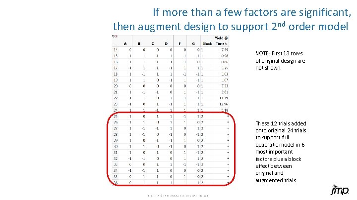
If more than a few factors are significant, then augment design to support 2 nd order model NOTE: First 13 rows of original design are not shown. These 12 trials added onto original 24 trials to support full quadratic model in 6 most important factors plus a block effect between original and augmented trials Copyright © SAS Inst itute Inc. All rig hts reserved.

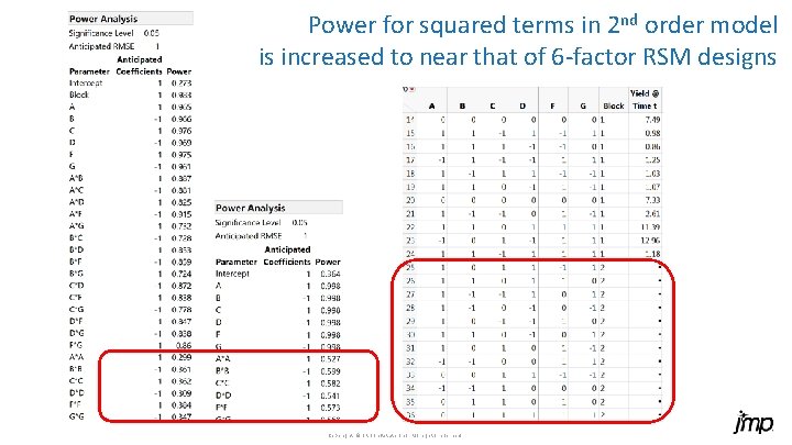
Power for squared terms in 2 nd order model is increased to near that of 6 -factor RSM designs Copyright © SAS Inst itute Inc. All rig hts reserved.

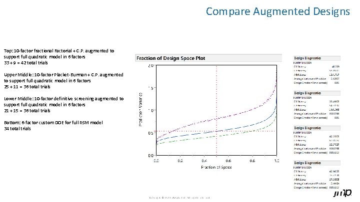
Compare Augmented Designs Top: 10 -factor fractional Factorial + C. P. augmented to support full quadratic model in 6 factors 33 + 9 = 42 total trials Upper Middle: 10 -factor Placket-Burman + C. P. augmented to support full quadratic model in 6 factors 25 + 11 = 36 total trials Lower Middle: 10 -factor definitive screening augmented to support full quadratic model in 6 factors 21 + 15 = 36 total trials Bottom: 6 -factor custom DOE for full RSM model 34 total trials Copyright © SAS Inst itute Inc. All rig hts reserved.

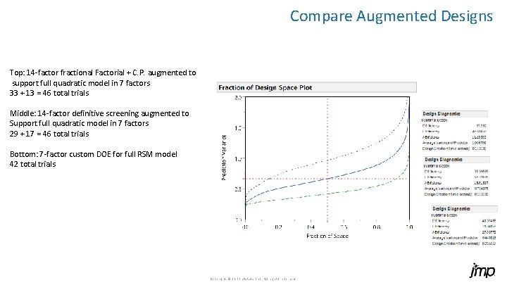
Compare Augmented Designs Top: 14 -factor fractional Factorial + C. P. augmented to support full quadratic model in 7 factors 33 + 13 = 46 total trials Middle: 14 -factor definitive screening augmented to Support full quadratic model in 7 factors 29 + 17 = 46 total trials Bottom: 7 -factor custom DOE for full RSM model 42 total trials Copyright © SAS Inst itute Inc. All rig hts reserved.

Number of Unique Trials for 3 Response-Surface Designs and Number of Quadratic Model Terms vs. Number of Continuous Factors Unique Trials in Central Composite Design Unique Trials in Box-Behnken Design Unique Trials in Custom Design with 6 df for Model Error Terms in Quadratic Model 36 trial I-optimal response-surface design started as 10 -factor DSD and was then augmented with 12 more trials in 6 most important factors If generally running 3, 4 or 5 -factor fractional-factorial designs… 1. How many interactions are you not investigating? 2. How many more trials needed to fit curvature? 3. Consider two stages: Definitive Screening + Augmentation Copyright © SAS Inst itute Inc. All rig hts reserved.

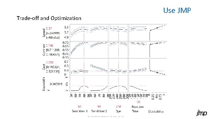
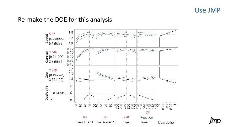
Use JMP Trade-off and Optimization Copyright © SAS Inst itute Inc. All rig hts reserved.

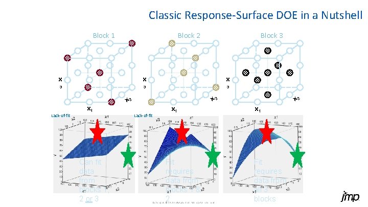
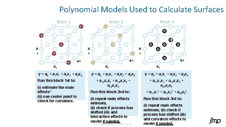
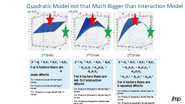
Classic Response-Surface DOE in a Nutshell Block 1 Block 2 Block 3 x x x 3 3 3 Lack-of-fit x 1 Can fit data from blocks 1, 2 or 3 x 2 x 2 Lack-of-fit x 1 Fit requires data from blocks 1 & 2 Copyright © SAS Inst itute Inc. All rig hts reserved. x 1 Fit requires data from all 3 blocks

Polynomial Models Used to Calculate Surfaces Block 1 Block 2 Block 3 x x x 3 3 3 x 1 y = a 0 + a 1 x 1 + a 2 x 2 + a 3 x 3 Run this block 1 st to: (i) estimate the main effects* (ii) use center point to check for curvature. x 2 x 2 x 1 y = a 0 + a 1 x 1 + a 2 x 2 + a 3 x 3 + a 12 x 1 x 2 + a 13 x 1 x 3 + a 23 x 2 x 3 Run this block 2 nd to: (i) repeat main effects estimate, (ii) check if process has shifted (iii) add interaction effects to model if needed. Copyright © SAS Inst itute Inc. All rig hts reserved. + a 11 x 12 + a 22 x 22 + a 33 x 32 Run this block 3 rd to: (i) repeat main effects estimate, (ii) check if process has shifted (iii) add curvature effects to model if needed.

Number of Unique Trials for 3 Response-Surface Designs and Number of Quadratic Model Terms vs. Number of Continuous Factors Unique Trials in Central Composite Design Unique Trials in Box-Behnken Design Unique Trials in Custom Design with 6 df for Model Error Terms in Quadratic Model If generally running 3, 4 or 5 -factor fractional-factorial designs… 1. How many interactions are you not investigating? 2. How many more trials needed to fit curvature? 3. Consider two stages: Definitive Screening + Augmentation Copyright © SAS Inst itute Inc. All rig hts reserved.

Classic Definition of DOE Purposeful control of the inputs (factors) in such a way as to deduce their relationships (if any) with the output (responses). Copyright © SAS Inst itute Inc. All rig hts reserved.

Alternative Definition of DOE A DOE is the specific collection of trials run to support a proposed model. § If proposed model is simple, e. g. just main effects or 1 st order effects (x 1 , x 2 , x 3, etc. ), the design is called a screening DOE » Goals include rank factor importance or find a “winner” quickly » Used with many (> 6? ) factors at start of process characterization § If the proposed model is more complex, e. g. the model is 2 nd order so that it includes two-way interaction terms (x 1 x 2 , x 1 x 3, x 2 x 3, etc. ) and in the case of continuous factors, squared terms (x 12, x 22, x 32 , etc. ), the design is called a response-surface DOE » Goal is generally to develop a predictive model of the process » Used with a few (< 6? ) factors after a screening DOE Copyright © SAS Inst itute Inc. All rig hts reserved.

Quadratic Model not that Much Bigger than Interaction Model Lack-of-fit Can fit data from blocks 1, 21 stor. Order 3 Fit requires data from blocks 1 & 22 nd Order Fit requires data from all 3 nd Order 2 blocks y = a 0 + a 1 x 1 + a 2 x 2 + a 3 x 3 + a 12 x 1 x 2 + a 13 x 1 x 3 + a 23 x 2 x 3 For k factors there are k main effects For 3 factors Linear Model has 4 terms For 6 factors Linear Model has 7 terms For 10 factors Linear Model has 11 terms For k factors there are k(k-1)/2 interaction effects For 3 factors Interaction Model has 7 terms For 6 factors Interaction Model has 22 terms For 10 factors Interaction has Copyright © SAS Inst itute Inc. All rig. Model hts reserved. + a 11 x 12 + a 22 x 22 + a 33 x 32 For k factors there are k squared effects For 3 factors Quadratic Model has 10 terms For 6 factors Quadratic Model has 28 terms For 10 factors Quadratic Model has 66

Use JMP Re-make the DOE for this analysis Copyright © SAS Inst itute Inc. All rig hts reserved.

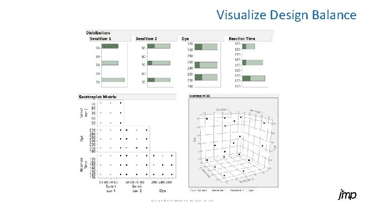
Visualize Design Balance Copyright © SAS Inst itute Inc. All rig hts reserved.