Special Class on RealTime Systems Realtime vs general

Special Class on Real-Time Systems

Real-time vs. general operating system • In addition to requiring logical correctness, real-time systems require temporal correctness – Logical correctness: Given an input, the system must create the correct output – Temporal correctness: The correct output must be created at the correct time

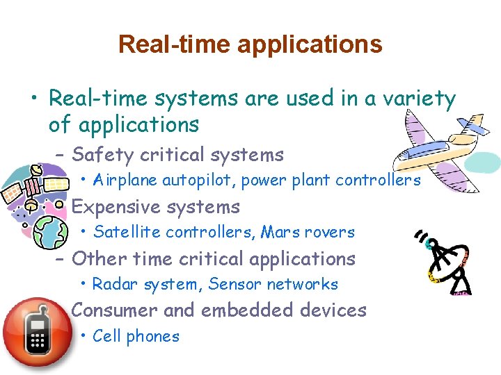
Real-time applications • Real-time systems are used in a variety of applications – Safety critical systems • Airplane autopilot, power plant controllers – Expensive systems • Satellite controllers, Mars rovers – Other time critical applications • Radar system, Sensor networks – Consumer and embedded devices • Cell phones

Aspects of real-time research • There are many active areas of research real-time systems – – – – Scheduling algorithms Schedulability tests Strategies for reducing power consumption Real-time operating systems Real-time programming languages Specific real-time applications Hardware for real-time systems

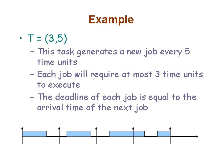
Standard real-time system model • Periodic tasks: A mechanism for executing a job repeatedly at regular time intervals – Example: Taking the temperature and initiating appropriate response in a power plant controller • T = (e, p) – e = execution requirement – p = period

Example • T = (3, 5) – This task generates a new job every 5 time units – Each job will require at most 3 time units to execute – The deadline of each job is equal to the arrival time of the next job

Task utilization • Given a periodic task T = (e, p), the utilization of T is e/p – Proportion of processing time this task will require on average • Many schedulability tests are based on task utilization

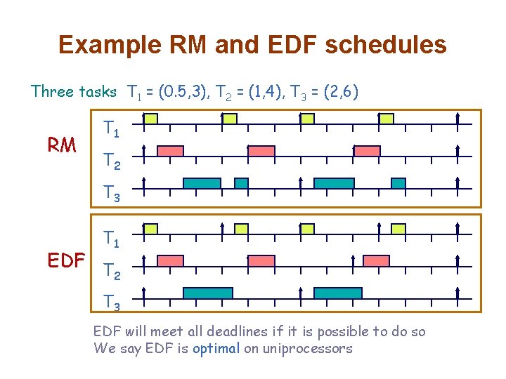
Two common scheduling algorithms • Earliest Deadline First (EDF) – Jobs with earlier deadlines are given higher priority • Rate Monotonic (RM) – Jobs generated by tasks with shorter periods are given higher priority

Example RM and EDF schedules Three tasks, T 1 = (0. 5, 3), T 2 = (1, 4), T 3 = (2, 6) RM T 1 T 2 T 3 T 1 EDF T 2 T 3 EDF will meet all deadlines if it is possible to do so We say EDF is optimal on uniprocessors

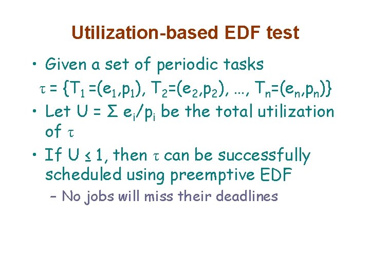
Utilization-based EDF test • Given a set of periodic tasks τ = {T 1 =(e 1, p 1), T 2=(e 2, p 2), …, Tn=(en, pn)} • Let U = Σ ei/pi be the total utilization of τ • If U ≤ 1, then τ can be successfully scheduled using preemptive EDF – No jobs will miss their deadlines

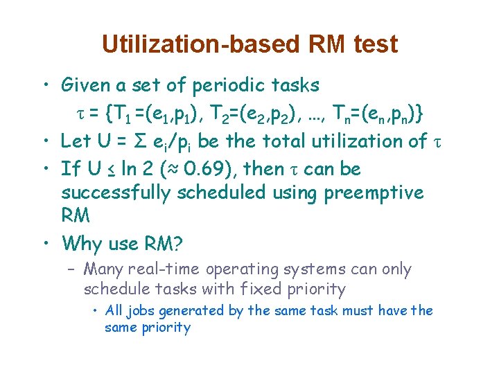
Utilization-based RM test • Given a set of periodic tasks τ = {T 1 =(e 1, p 1), T 2=(e 2, p 2), …, Tn=(en, pn)} • Let U = Σ ei/pi be the total utilization of τ • If U ≤ ln 2 (≈ 0. 69), then τ can be successfully scheduled using preemptive RM • Why use RM? – Many real-time operating systems can only schedule tasks with fixed priority • All jobs generated by the same task must have the same priority

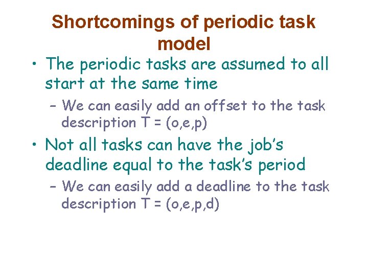
Shortcomings of periodic task model • The periodic tasks are assumed to all start at the same time – We can easily add an offset to the task description T = (o, e, p) • Not all tasks can have the job’s deadline equal to the task’s period – We can easily add a deadline to the task description T = (o, e, p, d)

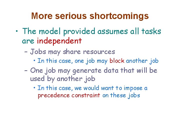
More serious shortcomings • The model provided assumes all tasks are independent – Jobs may share resources • In this case, one job may block another job – One job may generate data that will be used by another job • In this case, we would want to impose a precedence constraint on these jobs

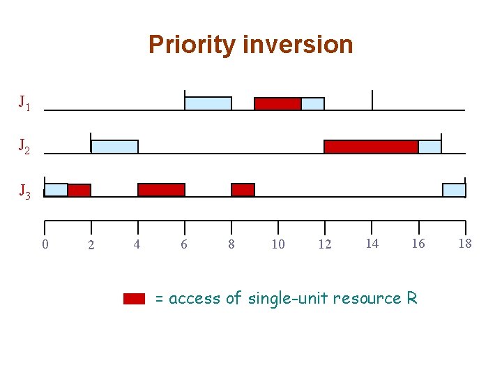
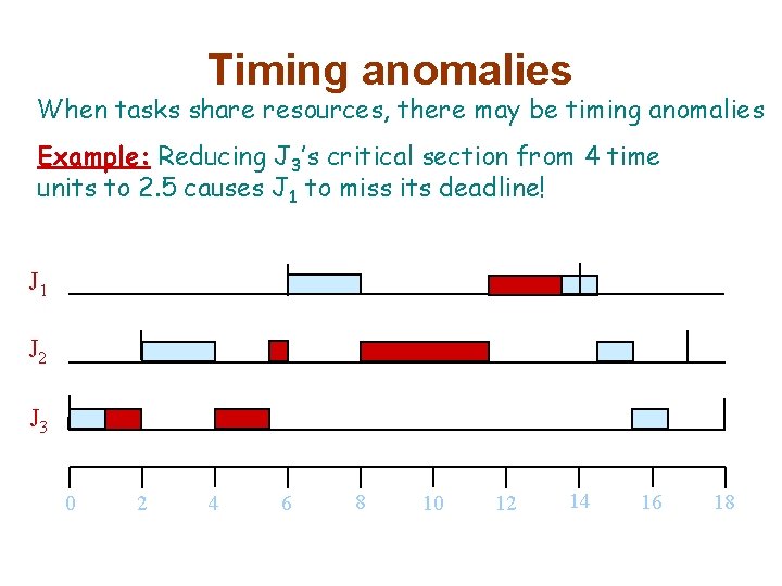
Scheduling jobs with dependiencies • Both blocking and precedence constraints can cause priority inversion and timing anomolies – Priority inversion: A higher priority job may be forced to wait while a lower priority job executes – Timing anomolies: Reducing the execution of one job may cause another job finish execution at a later time

Priority inversion J 1 J 2 J 3 0 2 4 6 8 10 12 14 16 = access of single-unit resource R 18

Timing anomalies When tasks share resources, there may be timing anomalies. Example: Reducing J 3’s critical section from 4 time units to 2. 5 causes J 1 to miss its deadline! J 1 J 2 J 3 0 2 4 6 8 10 12 14 16 18

Multiprocessor Scheduling • Scheduling analysis is much more difficult on multiprocessors • Many tests can only guarantee feasibility when the utilization is approximately m/2, where m is the number of processors – Things get even more complicated when there is resource sharing or precedence constraints

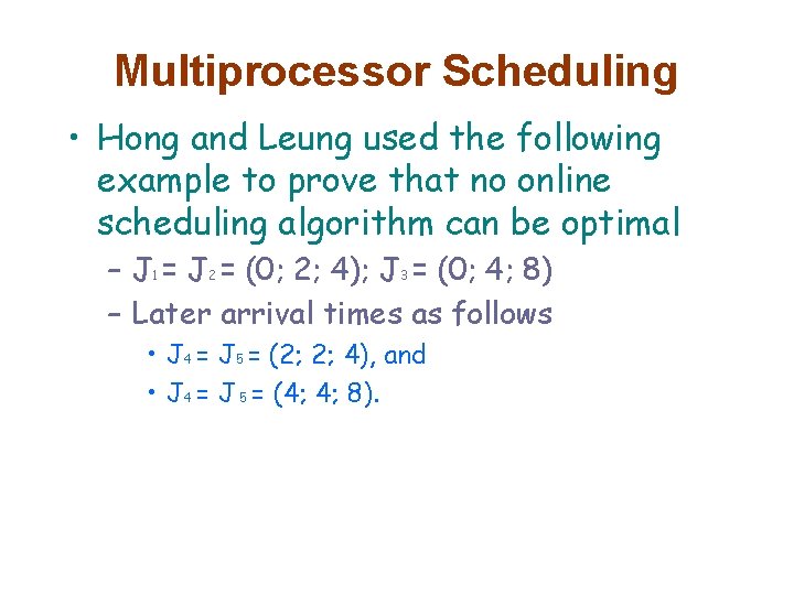
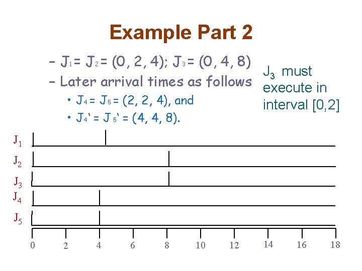
Multiprocessor Scheduling • Hong and Leung used the following example to prove that no online scheduling algorithm can be optimal – J 1 = J 2 = (0; 2; 4); J 3 = (0; 4; 8) – Later arrival times as follows • J 4 = J 5 = (2; 2; 4), and • J 4 = J 5 = (4; 4; 8).

Example Part 1 – J 1 = J 2 = (0, 2, 4); J 3 = (0, 4, 8) J 3 cannot – Later arrival times as follows execute in • J 4 = J 5 = (2, 2, 4), and interval [0, 2] • J 4‘ = J 5‘ = (4, 4, 8). J 1 J 2 J 3 J 4 J 5 0 2 4 6 8 10 12 14 16 18

Example Part 2 – J 1 = J 2 = (0, 2, 4); J 3 = (0, 4, 8) J 3 must – Later arrival times as follows execute in • J 4 = J 5 = (2, 2, 4), and interval [0, 2] • J 4‘ = J 5‘ = (4, 4, 8). J 1 J 2 J 3 J 4 J 5 0 2 4 6 8 10 12 14 16 18

Multiprocessor Scheduling of PTs • There are optimal online algorithms for scheduling periodic tasks on multiprocessors – Pfair, LLREF, DP-Wrap • These tasks make decisions to emulate the ideal schedule

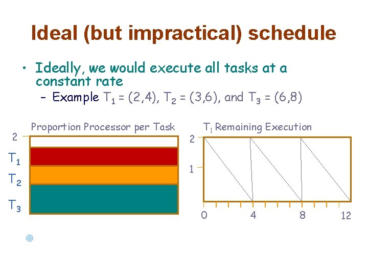
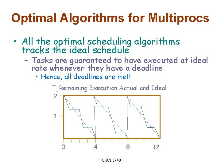
Ideal (but impractical) schedule • Ideally, we would execute all tasks at a constant rate – Example T 1 = (2, 4), T 2 = (3, 6), and T 3 = (6, 8) 2 Proportion Processor per Task T 1 2 T 1 Remaining Execution 1 T 2 T 3 0 ¥ 4 8 12 Unfortunately, there are only 2 processors and each can execute only one task at a time!

Optimal Algorithms for Multiprocs • All the optimal scheduling algorithms tracks the ideal schedule – Tasks are guaranteed to have executed at ideal rate whenever they have a deadline • Hence, all deadlines are met! T 1 Remaining Execution Actual and Ideal 2 1 0 4 8 CSCI 8740 12

DP-Fair Scheduling • A global scheduling algorithm for periodic tasks with deadlines equal to periods – The global scheduler executes whenever a job arrives / a deadline occurs • The intervals between scheduling events is called a time slice – At the beginning of each slice of length L, the scheduler allocates ui. L units of execution to each task Ti • Every DP-Fair Scheduling algorithm must adhere to 3 “don’t be stupid” rules

Don’t Be Stupid Rules • Rule 1: Execute any job with zero laxity – Execute right away if at risk of missing a deadline • Rule 2: Don’t execute any job with zero remaining execution time – Don’t execute if execution time is completed • Rule 3: Do not allow processors to idle for more than L(m – U) time units – Do not idle more than system slack allows

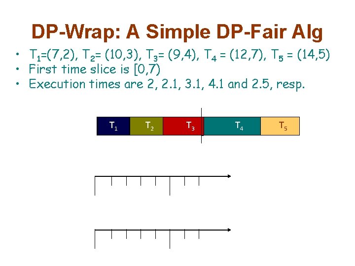
DP-Wrap: A Simple DP-Fair Alg • T 1=(7, 2), T 2= (10, 3), T 3= (9, 4), T 4 = (12, 7), T 5 = (14, 5) • First time slice is [0, 7) • Execution times are 2, 2. 1, 3. 1, 4. 1 and 2. 5, resp. T 1 TT 2 2 T 3 T 4 T 5 T 5

Extensions to the DP-Fair Rules • DP-Fair can also be used with sporadic tasks and tasks with deadlines not equal to periods – If deadlines are ≥ periods, DP-Fair algorithms are still optimal – If deadlines are < periods optimality no longer holds

Other types of real-time systems • Soft real-time systems – Deadlines may be missed • Mixed real-time and non-real-time sytems – Real-time and non-real-time jobs executing in the same system • Want non-real-time jobs to complete as early as possible without causing real-time jobs to miss deadlines

Why I like researching real-time systems • Analyzing real-time systems is like solving puzzles – Analysis is visual – Small changes in assumptions can have large impact in analysis