SPATIOTEMPORAL SCHEDULING FOR CROWD AUGMENTED URBAN SENSING Qiuxi

SPATIOTEMPORAL SCHEDULING FOR CROWD AUGMENTED URBAN SENSING Qiuxi Zhu, Md Yusuf Sarwar Uddin, Nalini Venkatasubramanian – Univ. California, Irvine, U. S. A. Cheng-Hsin Hsu – National Tsing Hua Univ. , Taiwan Funded by – CNS-1450768 MSE 446677 -22553

Motivation ■ Io. T helps achieve fine-grained urban sensing and monitoring – Environmental phenomena and human activities – In-situ and mobile devices – Diverse sensing capabilities ■ We anticipate that a large number of devices will participate in such activities in the near future. ■ Redundant data may lead to – Higher energy cost – Waste of network and cloud resources – Little contribution to accuracy 2

Spatiotemporal scheduling ■ Make plans for devices to regulate their sensing behavior (i. e. activate/deactivate their sensors) – Acceptable space-time coverage with limited data budget – Reduced redundancy ■ Challenges – Device heterogeneity: Availability of multiple sensor types – Data heterogeneity: Varying spatiotemporal requirements – Crowd mobility – Scalability: Number of devices and size of maps ■ Applicable to other geo-correlated data generation apps 3

Related work ■ Urban crowd-sensing S. Hachem (Per. Com ‘ 13) Y. Han (SECON ‘ 15) A. Khan (PMC, 2015) Y. Chen (Net. Games ‘ 17) M. Talasila (Mobi. CASE ‘ 14) TRAC (INFOCOM ‘ 14), etc. ■ Io. T and edge computing SCALE 2 (SMARTCOMP ‘ 16) H. Hong (Cloud. Com ‘ 17) ■ Pollution monitoring A. Marjovi (DCOSS ‘ 15) D. Hasenfratz (Per. Com ‘ 14) Y. Zheng (Ubi. Comp ‘ 14), etc. ■ Pollution severity R. Beelen, ’ 14 J. Zhang, ’ 14 N. Kunzli, ‘ 00 R. T. Burnett, ’ 00 X. Xu, ‘ 94 4

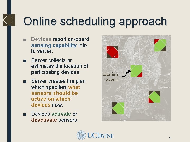
Online scheduling approach ■ Devices report on-board sensing capability info to server. ■ Server collects or estimates the location of participating devices. ■ Server creates the plan which specifies what sensors should be active on which devices now. This is a device ■ Devices activate or deactivate sensors. 5

Spatiotemporal scheduling ■ Problem formulation – Assumptions – Terms and notations – Spatiotemporal scheduling as multi-objective optimization ■ Online scheduling algorithms ■ Prototype platform and measurements ■ Performance evaluation and simulation results 6

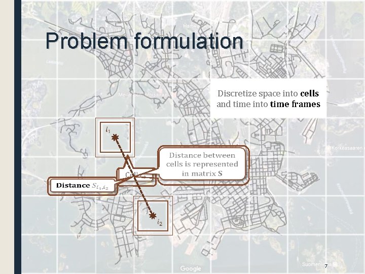
Problem formulation Discretize space into cells and time into time frames 7

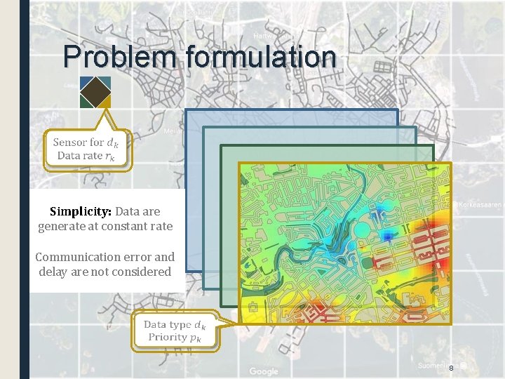
Problem formulation Simplicity: Data are generate at constant rate Communication error and delay are not considered 8

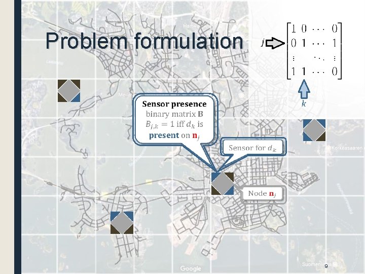
Problem formulation 9

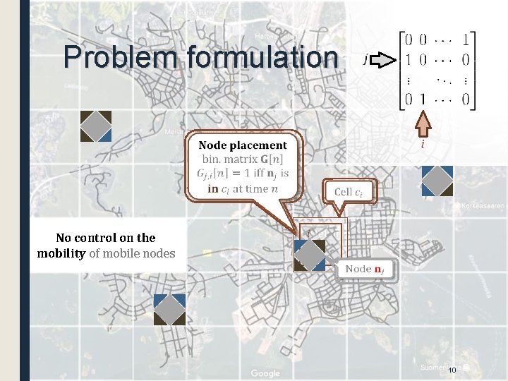
Problem formulation No control on the mobility of mobile nodes 10

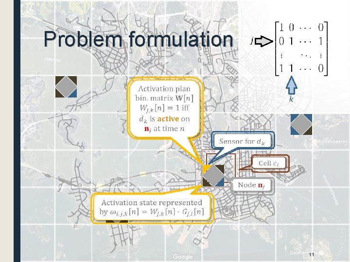
Problem formulation 11

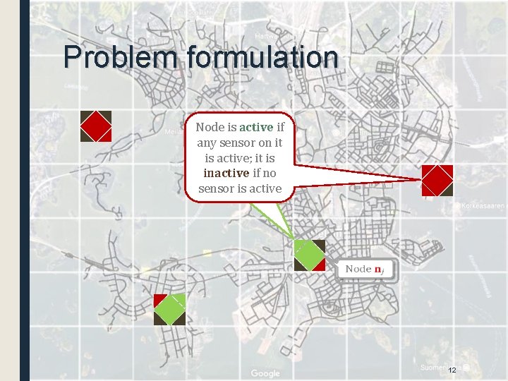
Problem formulation Node is active if any sensor on it is active; it is inactive if no sensor is active 12

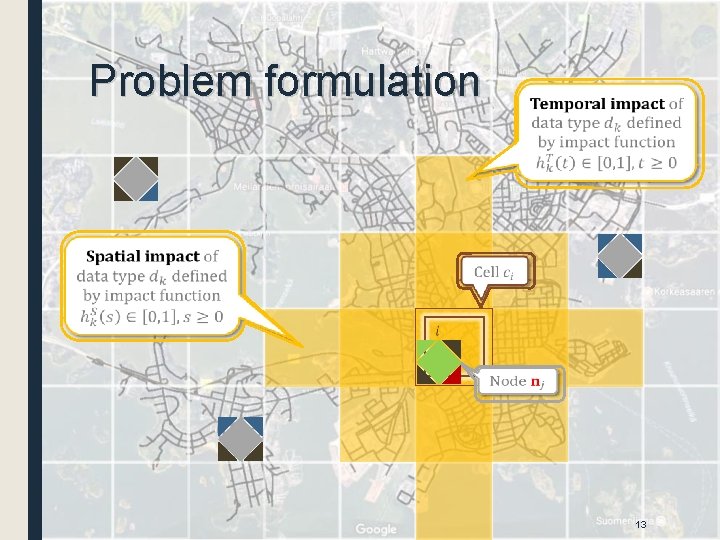
Problem formulation 13

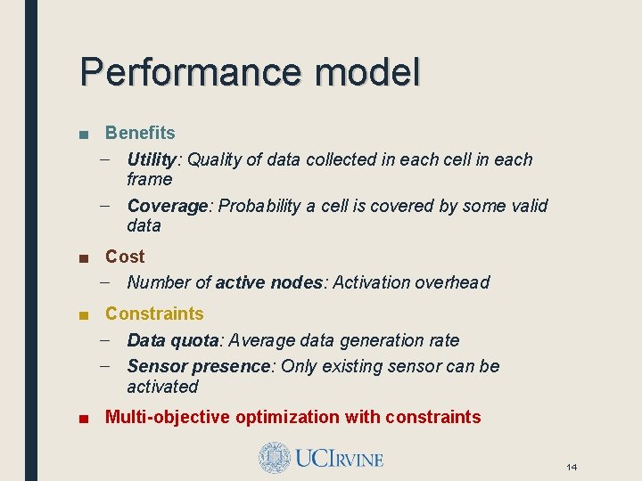
Performance model ■ Benefits – Utility: Quality of data collected in each cell in each frame – Coverage: Probability a cell is covered by some valid data ■ Cost – Number of active nodes: Activation overhead ■ Constraints – Data quota: Average data generation rate – Sensor presence: Only existing sensor can be activated ■ Multi-objective optimization with constraints 14

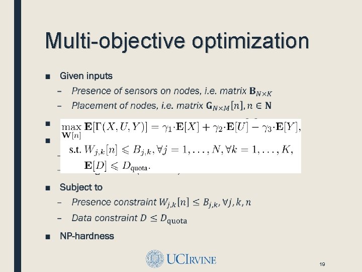
Multi-objective optimization ■ 19

Spatiotemporal scheduling ■ Problem formulation – Assumptions – Terms and notations – Spatiotemporal scheduling as multi-objective optimization ■ Online scheduling algorithms ■ Prototype platform and measurements ■ Performance evaluation and simulation results 20

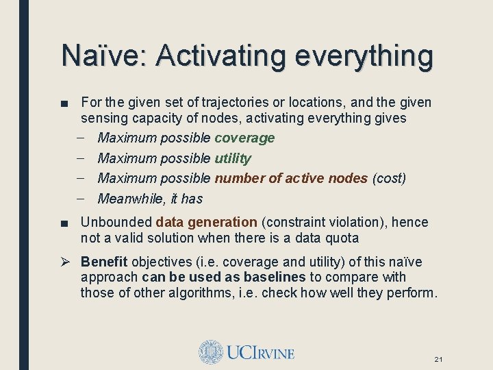
Naïve: Activating everything ■ For the given set of trajectories or locations, and the given sensing capacity of nodes, activating everything gives – Maximum possible coverage – Maximum possible utility – Maximum possible number of active nodes (cost) – Meanwhile, it has ■ Unbounded data generation (constraint violation), hence not a valid solution when there is a data quota Ø Benefit objectives (i. e. coverage and utility) of this naïve approach can be used as baselines to compare with those of other algorithms, i. e. check how well they perform. 21

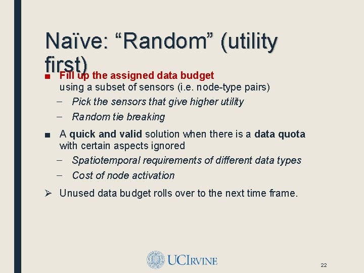
Naïve: “Random” (utility first) ■ Fill up the assigned data budget using a subset of sensors (i. e. node-type pairs) – Pick the sensors that give higher utility – Random tie breaking ■ A quick and valid solution when there is a data quota with certain aspects ignored – Spatiotemporal requirements of different data types – Cost of node activation Ø Unused data budget rolls over to the next time frame. 22

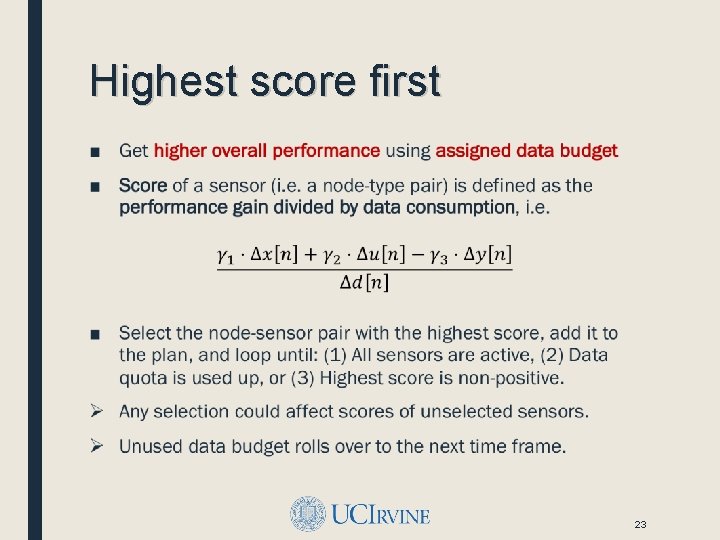
Highest score first ■ 23

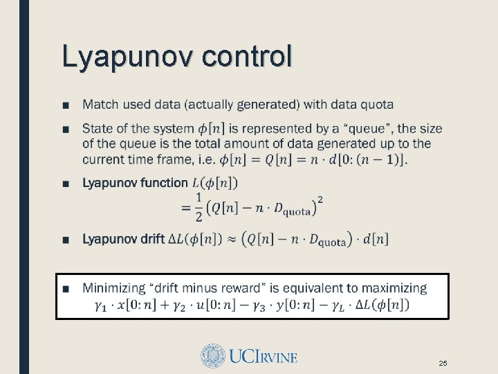
Lyapunov control ■ 25

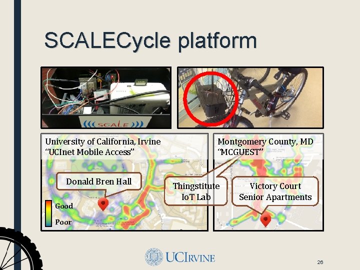
SCALECycle platform University of California, Irvine “UCInet Mobile Access” Donald Bren Hall Good Montgomery County, MD “MCGUEST” Thingstitute Io. T Lab Victory Court Senior Apartments Poor 26

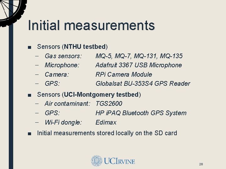
Initial measurements ■ Sensors (NTHU testbed) – Gas sensors: MQ-5, MQ-7, MQ-131, MQ-135 – Microphone: Adafruit 3367 USB Microphone – Camera: RPi Camera Module – GPS: Globalsat BU-353 S 4 GPS Reader ■ Sensors (UCI-Montgomery testbed) – Air contaminant: TGS 2600 – GPS: HP i. PAQ Bluetooth GPS System – Wi-Fi dongle: Edimax ■ Initial measurements stored locally on the SD card 28

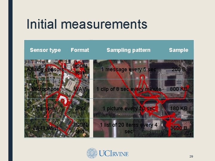
Initial measurements Montgomery County, MD Sensor type Format NTHU Campus, Hsinchu City, Taiwan Sampling pattern Sample Analog sensors JSON text 1 message every 5 sec 200 B Microphone WAV 1 clip of 8 sec every minute 800 KB Camera JPG 1 picture every 20 sec 180 KB Wi-Fi iwlist JSON text 1 list of 20 items every 4 sec 3600 B 29

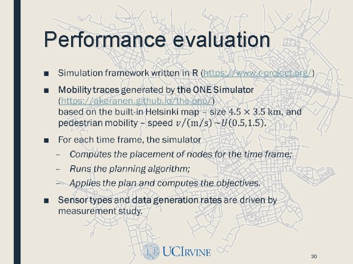
Performance evaluation ■ 30

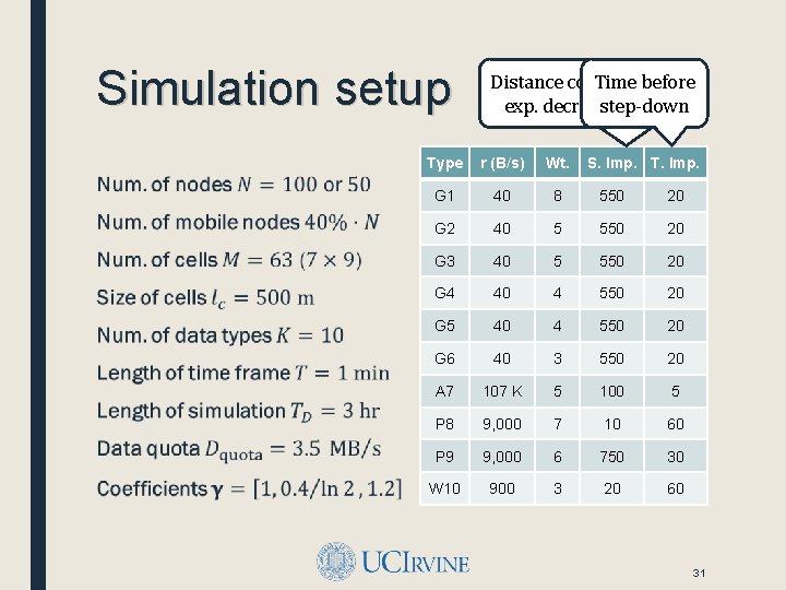
Simulation setup ■ Distance coefficient Time before of exp. decrease step-down func. Type r (B/s) Wt. S. Imp. T. Imp. G 1 40 8 550 20 G 2 40 5 550 20 G 3 40 5 550 20 G 4 40 4 550 20 G 5 40 4 550 20 G 6 40 3 550 20 A 7 107 K 5 100 5 P 8 9, 000 7 10 60 P 9 9, 000 6 750 30 W 10 900 3 20 60 31

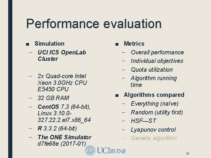
Performance evaluation ■ Simulation – UCI ICS Open. Lab Cluster – 2 x Quad-core Intel Xeon 3. 0 GHz CPU E 5450 CPU – 32 GB RAM – Cent. OS 7. 3 (64 -bit), Linux 3. 10. 0327. 22. 2. el 7. x 86_64 – R 3. 3. 2 (64 -bit) – The ONE Simulator d 7 fe 68 e (2017 -01) ■ Metrics – Overall performance – Individual objectives – Quota utilization – Algorithm running time ■ Algorithms compared – Everything (naïve) – Random (utility first) – HSF—ST – Lyapunov control – Genetic algorithm 32

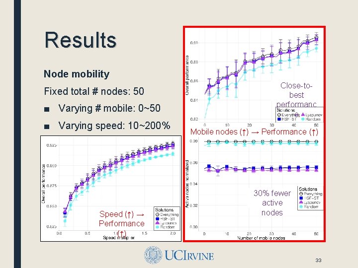
Results Node mobility Fixed total # nodes: 50 ■ Varying # mobile: 0~50 ■ Varying speed: 10~200% Speed (↑) → Performance (↑) Close-tobest performanc e Mobile nodes (↑) → Performance (↑) 30% fewer active nodes 33

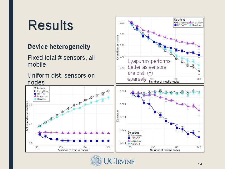
Results Device heterogeneity Fixed total # sensors, all mobile Uniform dist. sensors on nodes Lyapunov performs better as sensors are dist. (↑) sparsely ■ Varying # nodes: 50~200 34

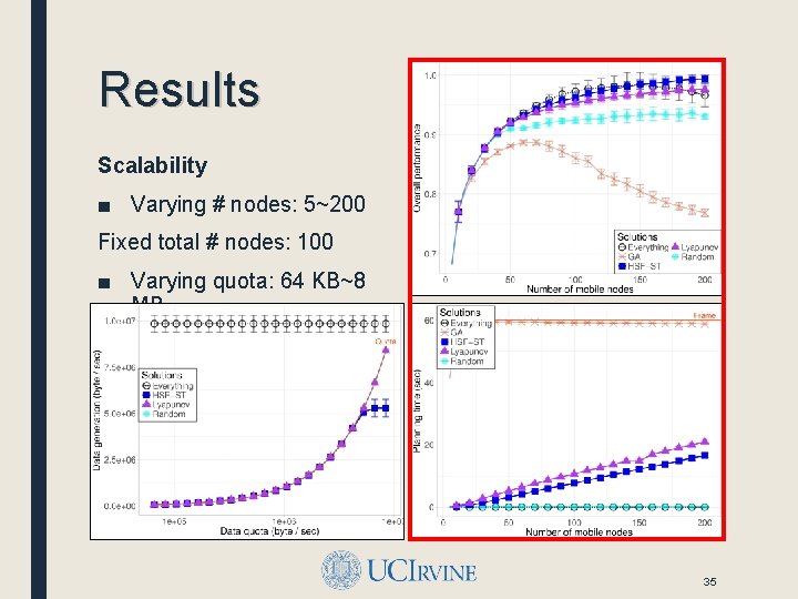
Results Scalability ■ Varying # nodes: 5~200 Fixed total # nodes: 100 ■ Varying quota: 64 KB~8 MB 35

Conclusion ■ Contributions – Motivated and formalized the spatiotemporal scheduling problem for crowd-augmented urban sensing; – Proposed an online framework and two algorithms; – Conducted measurement-driven simulations showing the effectiveness of proposed approach. ■ Achieved similar coverage (comparing to “everything”) under data constraints, with about 30% fewer active nodes. ■ Future works – Improve scalability with scheduling hierarchies – Study impact of network connectivity and uncertainty 36

Questions? ■ Distributed Systems Middleware (DSM) Group at UCI http: //www. ics. uci. edu/~dsm/ ■ Information Systems Group (ISG) at UCI https: //isg. ics. uci. edu/ ■ Networking and Multimedia Systems Lab (NMSL) at NTHU https: //nmsl. cs. nthu. edu. tw/ ■ Safe Community Awareness and Alerting (SCALE) Project http: //scale. ics. uci. edu/ ■ Qiuxi Zhu https: //sites. google. com/site/zhuqiuxiuci 37

SPATIOTEMPORAL SCHEDULING FOR CROWD AUGMENTED URBAN SENSING Thank you! Email: qiuxiz <at> ics <dot> uci <dot> edu Funded by – CNS-1450768 MSE 446677 -22553