Spatial Subdivision Graham Rhodes Senior Software Developer Applied

Spatial Subdivision Graham Rhodes Senior Software Developer, Applied Research Associates, Inc.

How do you find a needle in a haystack? Image is in the public domain. Painting date 1874. File source is http: //commons. wikimedia. org/wiki/File: Haystacks_Autumn_1873_Jean-Francois_Millet. jpg 2

Spatial subdivision: what is it? ● A structured partitioning of geometry Y X 4

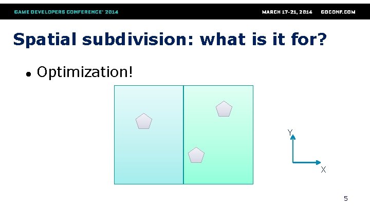
Spatial subdivision: what is it for? ● Optimization! Y X 5

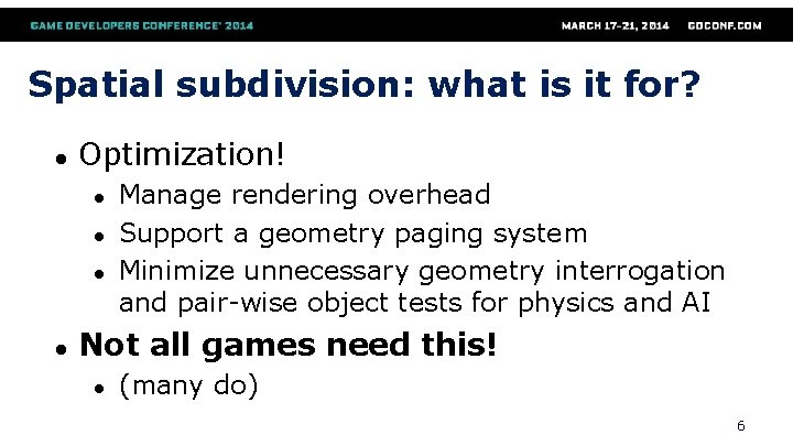
Spatial subdivision: what is it for? ● Optimization! ● ● Manage rendering overhead Support a geometry paging system Minimize unnecessary geometry interrogation and pair-wise object tests for physics and AI Not all games need this! ● (many do) 6

Classes of spatial subdivision ● ● ● Grid-based Tree-based Others ● ● ● Bounding Volume Hierarchy Scene Graph Portals 7

Grid-based Spatial Subdivision 8

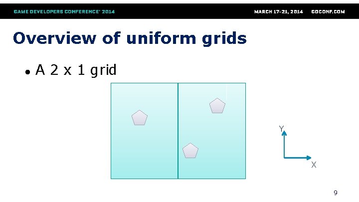
Overview of uniform grids ● A 2 x 1 grid Y X 9

Overview of uniform grids ● A 2 x 2 grid Y X 10

Overview of uniform grids ● A 4 x 3 grid Y X 11

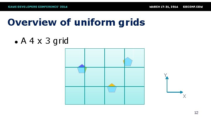
Overview of uniform grids ● A 4 x 3 grid Y X 12

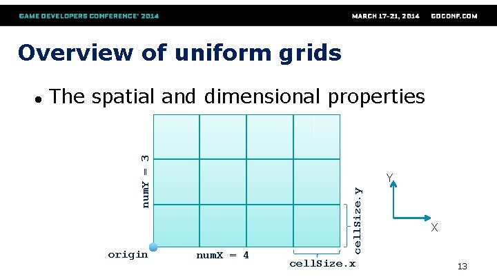
Overview of uniform grids The spatial and dimensional properties num. Y = 3 origin Y num. X = 4 cell. Size. y ● cell. Size. x X 13

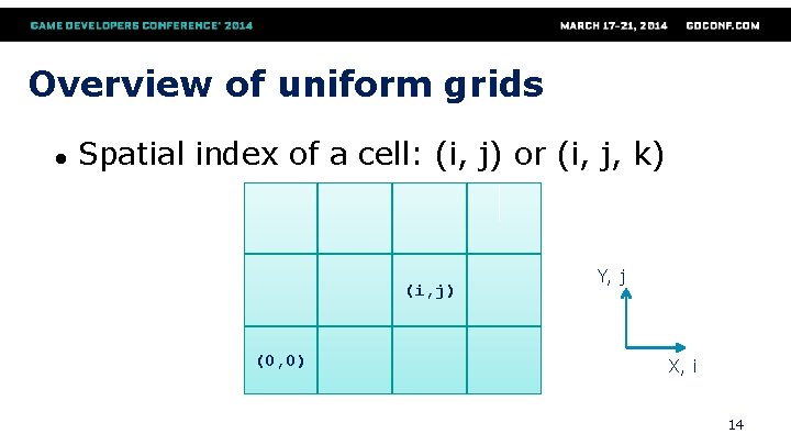
Overview of uniform grids ● Spatial index of a cell: (i, j) or (i, j, k) (i, j) (0, 0) Y, j X, i 14

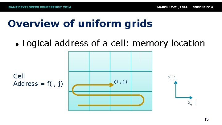
Overview of uniform grids ● Logical address of a cell: memory location Cell Address = f(i, j) Y, j X, i 15

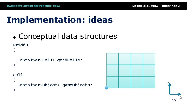
Implementation: ideas ● Conceptual data structures Grid 2 D { … Container<Cell> grid. Cells; } Cell { Container<Object> game. Objects; } Y 16 X

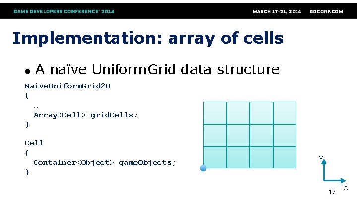
Implementation: array of cells ● A naïve Uniform. Grid data structure Naive. Uniform. Grid 2 D { … Array<Cell> grid. Cells; } Cell { Container<Object> game. Objects; } Y 17 X

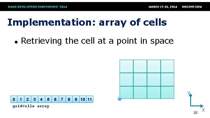
Implementation: array of cells ● Retrieving the cell at a point in space Y 0 1 2 3 4 5 6 7 8 9 10 11 grid. Cells array 18 X

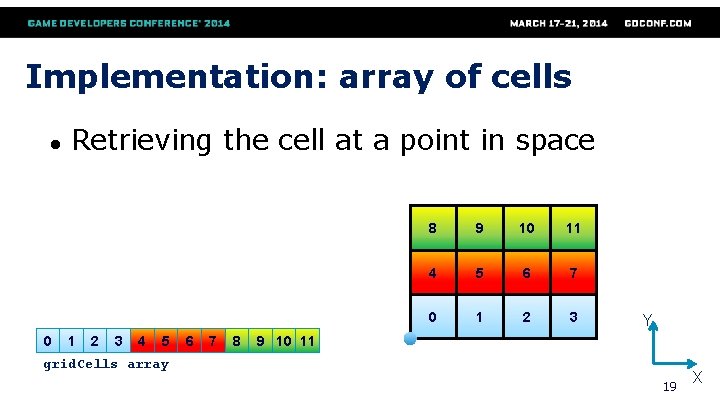
Implementation: array of cells ● 0 Retrieving the cell at a point in space 1 2 3 4 5 6 7 8 8 9 10 11 4 5 6 7 0 1 2 3 Y 9 10 11 grid. Cells array 19 X

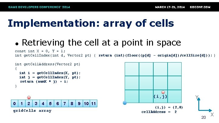
Implementation: array of cells ● Retrieving the cell at a point in space const int X = 0, Y = 1; int get. Cell. Index(int d, Vector 2 pt) { return (int)(floor((p[d] – origin[d])/cell. Size[d])); } int get. Cell. Address(Vector 2 pt) { int i = get. Cell. Index(X, pt); int j = get. Cell. Index(Y, pt); return (num. X * j) + i; } (i, j) 0 1 2 3 4 5 grid. Cells array 6 7 8 9 10 11 Y (i, j) = (2, 0) cell. Address = 2 20 X

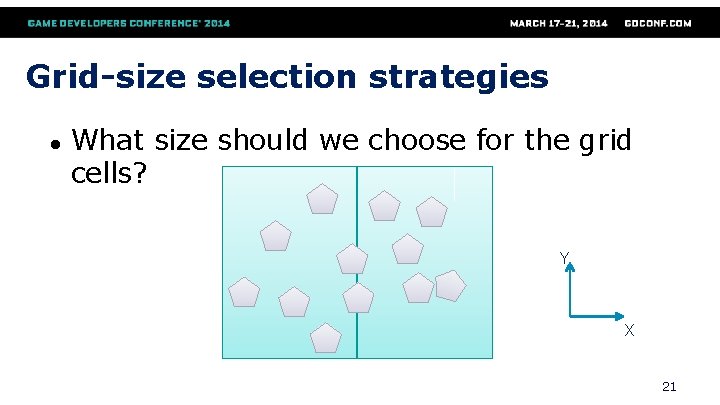
Grid-size selection strategies ● What size should we choose for the grid cells? Y X 21

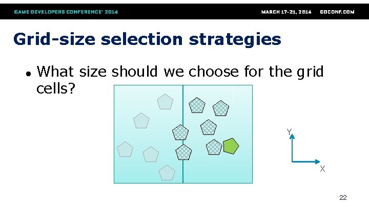
Grid-size selection strategies ● What size should we choose for the grid cells? Y X 22

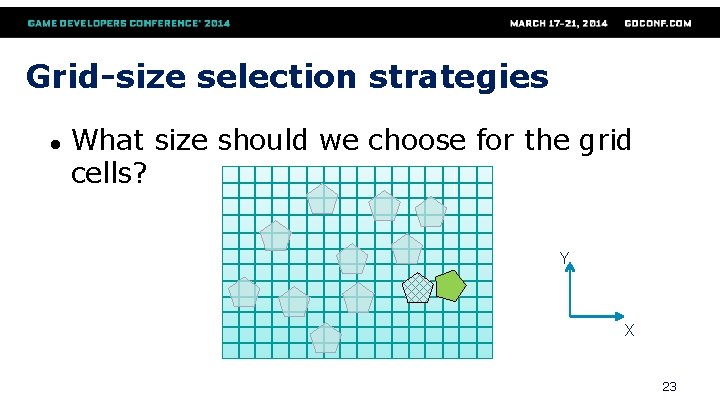
Grid-size selection strategies ● What size should we choose for the grid cells? Y X 23

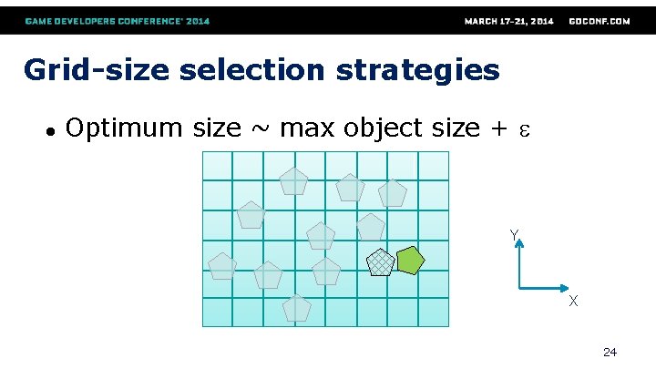
Grid-size selection strategies ● Optimum size ~ max object size + e Y X 24

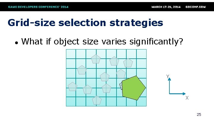
Grid-size selection strategies ● What if object size varies significantly? Y X 25

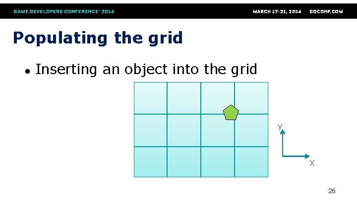
Populating the grid ● Inserting an object into the grid Y X 26

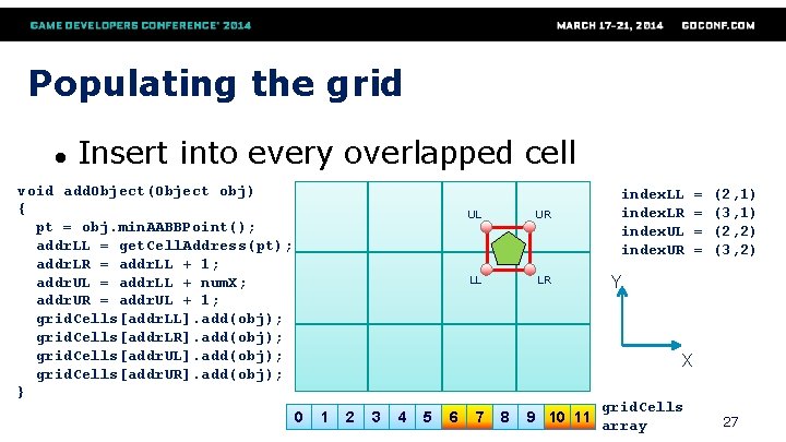
Populating the grid ● Insert into every overlapped cell void add. Object(Object obj) { pt = obj. min. AABBPoint(); addr. LL = get. Cell. Address(pt); addr. LR = addr. LL + 1; addr. UL = addr. LL + num. X; addr. UR = addr. UL + 1; grid. Cells[addr. LL]. add(obj); grid. Cells[addr. LR]. add(obj); grid. Cells[addr. UL]. add(obj); grid. Cells[addr. UR]. add(obj); } UL UR LL LR index. LL index. LR index. UL index. UR = = (2, 1) (3, 1) (2, 2) (3, 2) Y X 0 1 2 3 4 5 6 7 8 grid. Cells 9 10 11 array 27

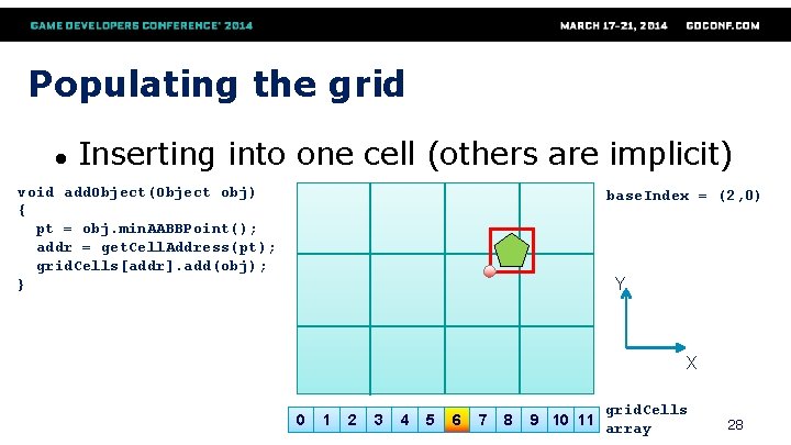
Populating the grid ● Inserting into one cell (others are implicit) void add. Object(Object obj) { pt = obj. min. AABBPoint(); addr = get. Cell. Address(pt); grid. Cells[addr]. add(obj); } base. Index = (2, 0) Y X 0 1 2 3 4 5 6 7 8 grid. Cells 9 10 11 array 28

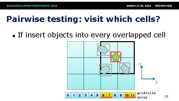
Pairwise testing: visit which cells? ● If insert objects into every overlapped cell Y X 0 1 2 3 4 5 6 7 8 grid. Cells 9 10 11 array 29

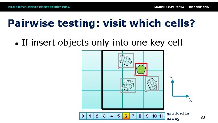
Pairwise testing: visit which cells? ● If insert objects only into one key cell Y X 0 1 2 3 4 5 6 7 8 grid. Cells 9 10 11 array 30

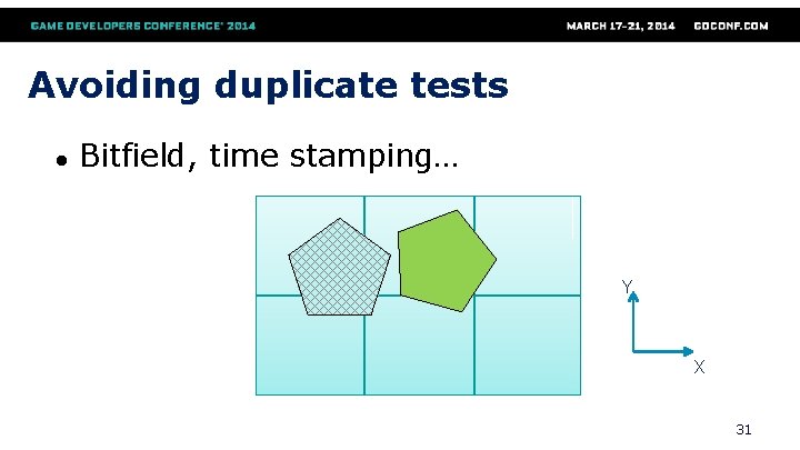
Avoiding duplicate tests ● Bitfield, time stamping… Y X 31

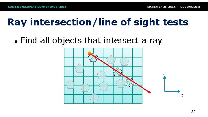
Ray intersection/line of sight tests ● Find all objects that intersect a ray Y X 32

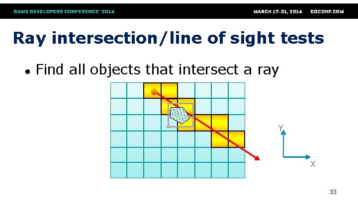
Ray intersection/line of sight tests ● Find all objects that intersect a ray Y X 33

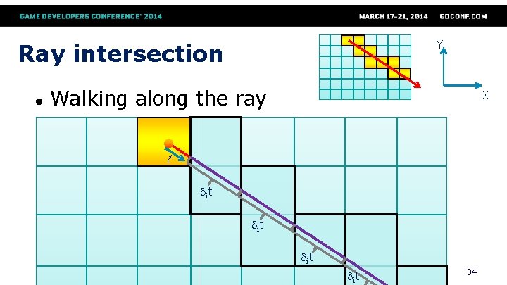
Y Ray intersection ● Walking along the ray X t dit dit 34

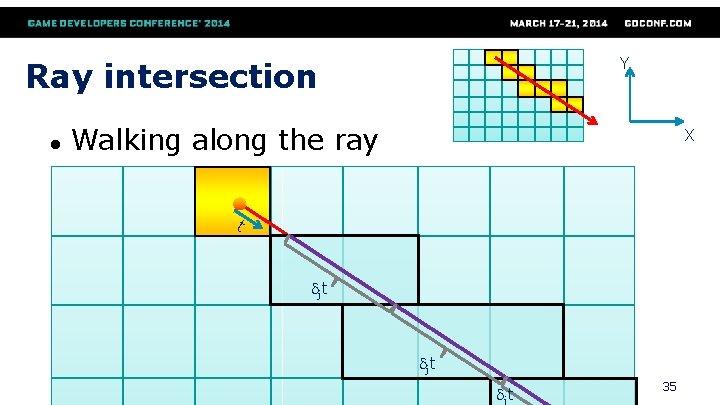
Y Ray intersection ● Walking along the ray X t djt djt 35

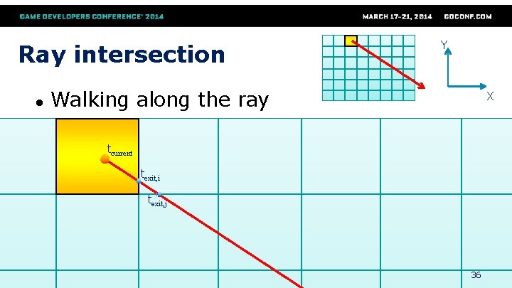
Ray intersection ● Y Walking along the ray X tcurrent texit, i texit, j 36

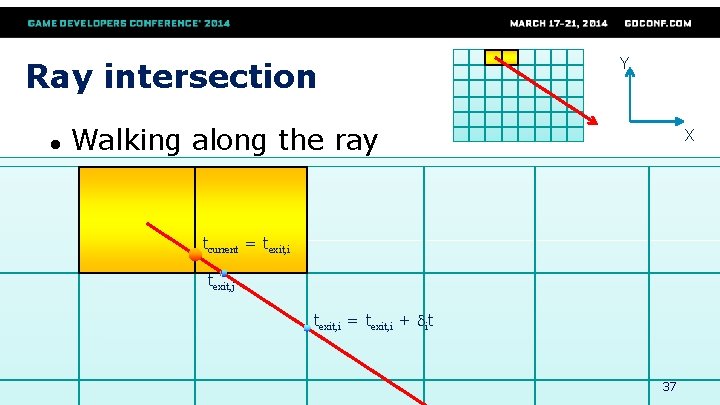
Ray intersection ● Y Walking along the ray X tcurrent = texit, i texit, j texit, i = texit, i + dit 37

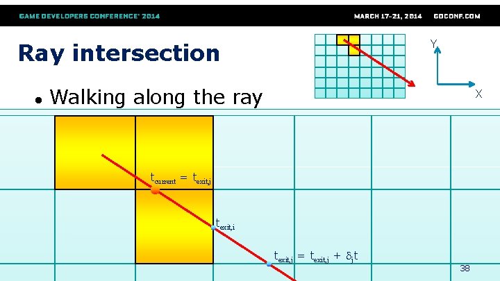
Y Ray intersection ● Walking along the ray X tcurrent = texit, j texit, i texit, j = texit, j + djt 38

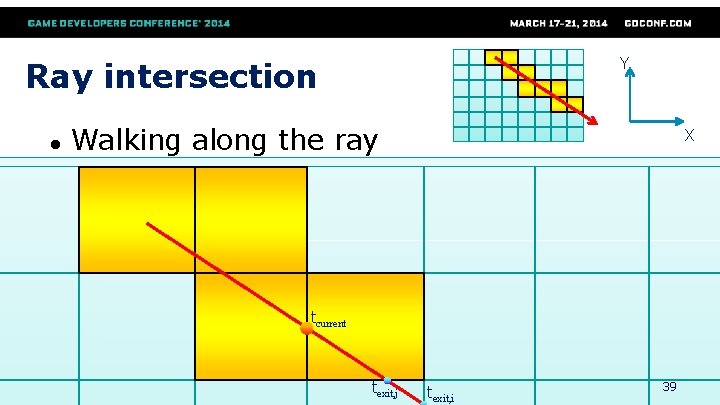
Y Ray intersection ● Walking along the ray X tcurrent texit, j texit, i 39

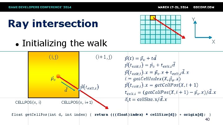
Ray intersection ● Y Initializing the walk (i+1, j) (i, j) CELLPOS(x, i+1) float get. Cell. Pos(int d, int index) { return (((float)index) * cell. Size[d]) + origin[d]; } 40 X

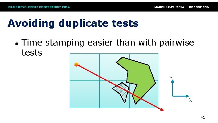
Avoiding duplicate tests ● Time stamping easier than with pairwise tests Y X 41

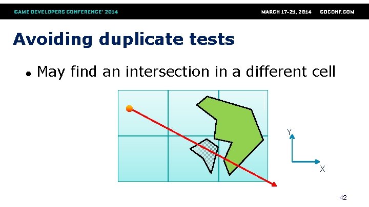
Avoiding duplicate tests ● May find an intersection in a different cell Y X 42

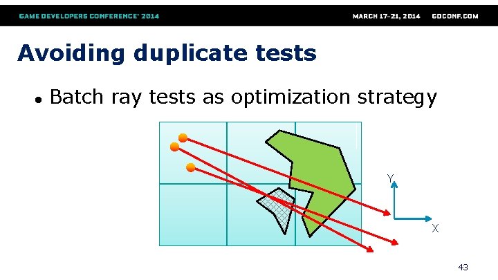
Avoiding duplicate tests ● Batch ray tests as optimization strategy Y X 43

Back to array of cells ● Does anyone see a problem with this naïve approach? ● ● ● Most cells are likely empty Doesn’t scale well due in part to large memory requirements For these reasons, this naïve array of cells approach is often a bad choice in practice 44

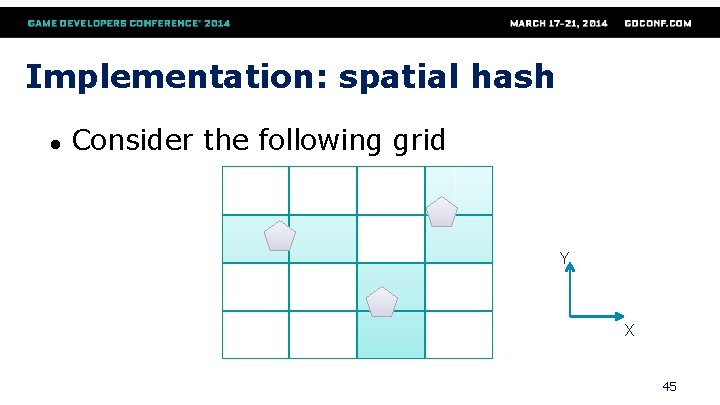
Implementation: spatial hash ● Consider the following grid Y X 45

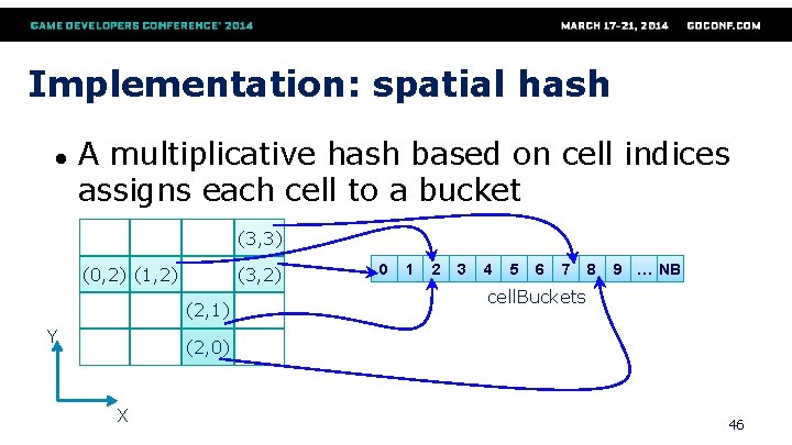
Implementation: spatial hash ● A multiplicative hash based on cell indices assigns each cell to a bucket (3, 3) (0, 2) (1, 2) (3, 2) (2, 1) Y 0 1 2 3 4 5 6 7 8 9 … NB cell. Buckets (2, 0) X 46

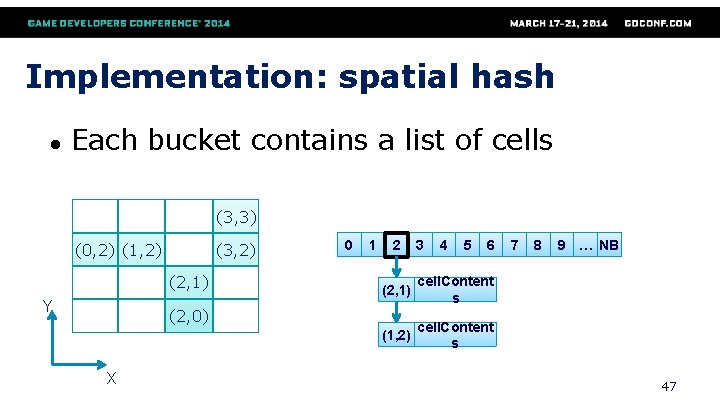
Implementation: spatial hash ● Each bucket contains a list of cells (3, 3) (0, 2) (1, 2) (3, 2) (2, 1) Y 0 1 2 4 5 6 (2, 1) cell. Content s (1, 2) cell. Content s (2, 0) X 3 7 8 9 … NB 47

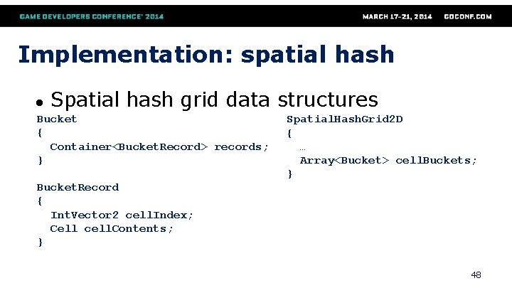
Implementation: spatial hash ● Spatial hash grid data structures Bucket { Container<Bucket. Record> records; } Spatial. Hash. Grid 2 D { … Array<Bucket> cell. Buckets; } Bucket. Record { Int. Vector 2 cell. Index; Cell cell. Contents; } 48

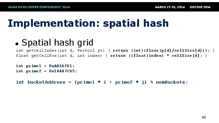
Implementation: spatial hash ● Spatial hash grid int get. Cell. Index(int d, Vector 2 pt) { return (int)(floor(p[d]/cell. Size[d])); } float get. Cell. Pos(int d, int index) { return ((float)index) * cell. Size[d]; } int prime 1 = 0 x. AB 1 D 261; int prime 2 = 0 x 16447 CD 5; int bucket. Address = (prime 1 * i + prime 2 * j) % num. Buckets; 49

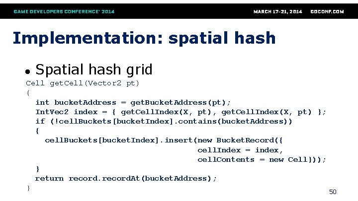
Implementation: spatial hash ● Spatial hash grid Cell get. Cell(Vector 2 pt) { int bucket. Address = get. Bucket. Address(pt); Int. Vec 2 index = { get. Cell. Index(X, pt), get. Cell. Index(X, pt) }; if (!cell. Buckets[bucket. Index]. contains(bucket. Address)) { cell. Buckets[bucket. Index]. insert(new Bucket. Record({ cell. Index = index, cell. Contents = new Cell})); } return record. At(bucket. Address); } 50

Tree-based Spatial Subdivision 51

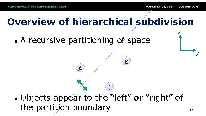
Overview of hierarchical subdivision ● A recursive partitioning of space Y X B A C ● Objects appear to the “left” or “right” of the partition boundary 52

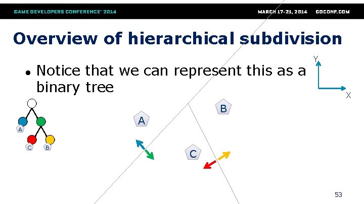
Overview of hierarchical subdivision ● Notice that we can represent this as a binary tree C B X B A A Y C 53

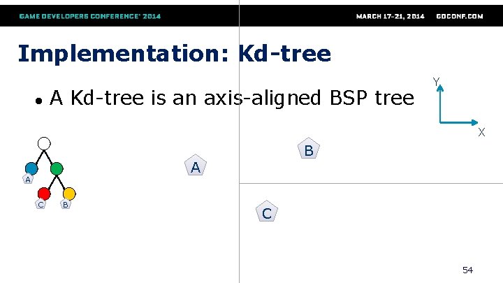
Implementation: Kd-tree ● A Kd-tree is an axis-aligned BSP tree Y X B A A C B C 54

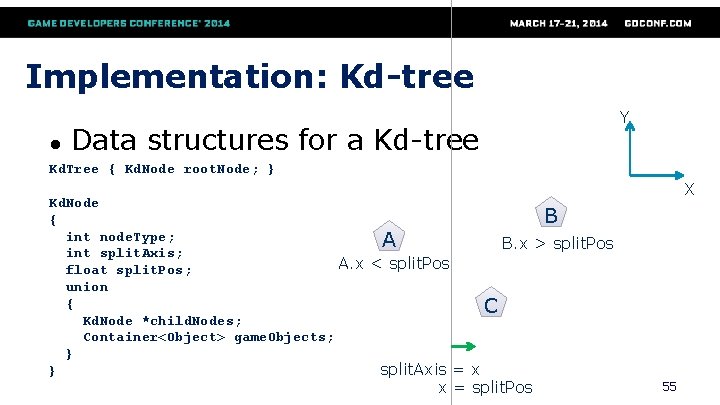
Implementation: Kd-tree ● Data structures for a Kd-tree Y Kd. Tree { Kd. Node root. Node; } Kd. Node B { int node. Type; A B. x > split. Pos int split. Axis; A. x < split. Pos float split. Pos; union { C Kd. Node *child. Nodes; Container<Object> game. Objects; } split. Axis = x } x = split. Pos X 55

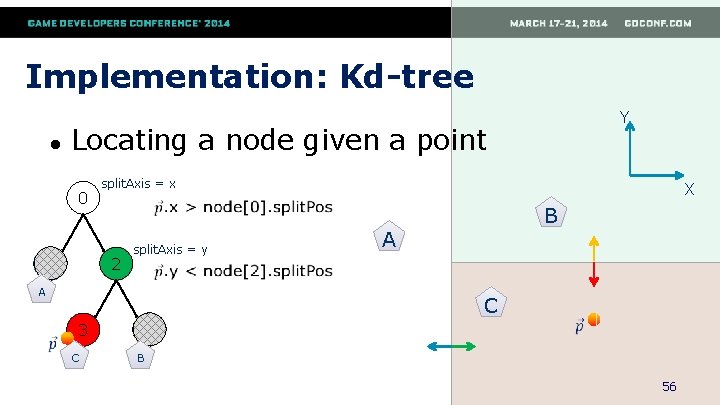
Implementation: Kd-tree ● Y Locating a node given a point 0 1 split. Axis = x 2 split. Axis = y A X B A C 3 C 4 B 56

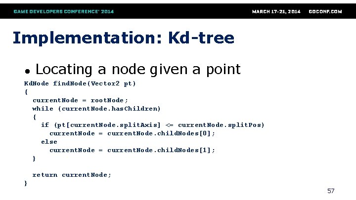
Implementation: Kd-tree ● Locating a node given a point Kd. Node find. Node(Vector 2 pt) { current. Node = root. Node; while (current. Node. has. Children) { if (pt[current. Node. split. Axis] <= current. Node. split. Pos) current. Node = current. Node. child. Nodes[0]; else current. Node = current. Node. child. Nodes[1]; } return current. Node; } 57

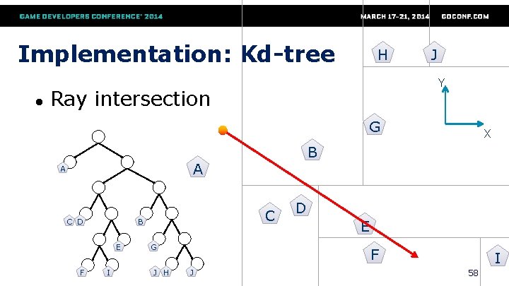
Implementation: Kd-tree ● H J Y Ray intersection G B A A C D E F C B I G J H X D E F J I 58

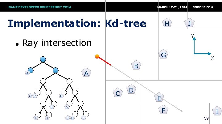
Implementation: Kd-tree ● H J Y Ray intersection G B A A C D E F C B I G J H X D E F J I 59

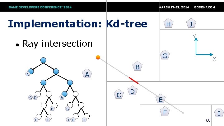
Implementation: Kd-tree ● H J Y Ray intersection G B A A C D E F C B I G J H X D E F J I 60

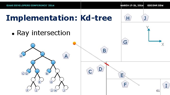
Implementation: Kd-tree ● H J Y Ray intersection G B A A C D E F C B I G J H X D E F J I 61

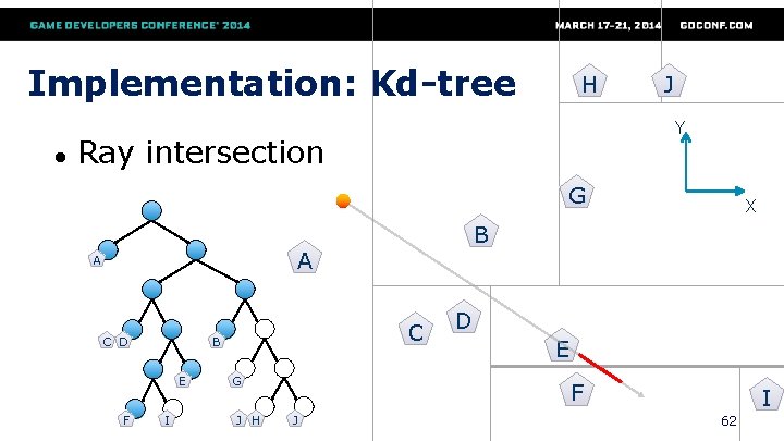
Implementation: Kd-tree ● H J Y Ray intersection G B A A C D E F C B I G J H X D E F J I 62

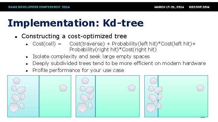
Implementation: Kd-tree ● Constructing a cost-optimized tree ● ● Cost(cell) = Cost(traverse) + Probability(left hit)*Cost(left hit)+ Probability(right hit)*Cost(right hit) Isolate complexity and seek large empty spaces Deeply subdivided trees tend to be more efficient on modern hardware Profile performance for your use case 63

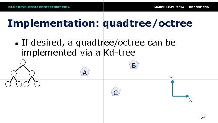
Implementation: quadtree/octree ● If desired, a quadtree/octree can be implemented via a Kd-tree B A Y C X 64

Problems with hierarchical subdivision ● Not suitable for dynamic/moving objects 65

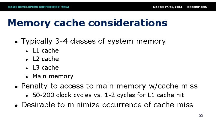
Memory cache considerations ● Typically 3 -4 classes of system memory ● ● ● Penalty to access to main memory w/cache miss ● ● L 1 cache L 2 cache L 3 cache Main memory 50 -200 clock cycles vs. 1 -2 cycles for L 1 cache hit Desirable to minimize occurrence of cache miss 66

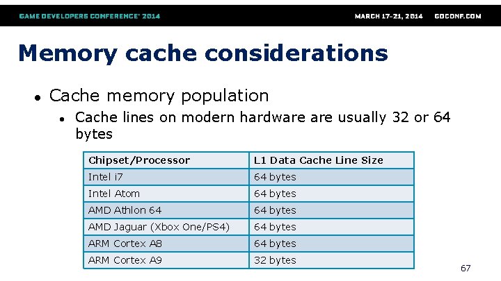
Memory cache considerations ● Cache memory population ● Cache lines on modern hardware usually 32 or 64 bytes Chipset/Processor L 1 Data Cache Line Size Intel i 7 64 bytes Intel Atom 64 bytes AMD Athlon 64 64 bytes AMD Jaguar (Xbox One/PS 4) 64 bytes ARM Cortex A 8 64 bytes ARM Cortex A 9 32 bytes 67

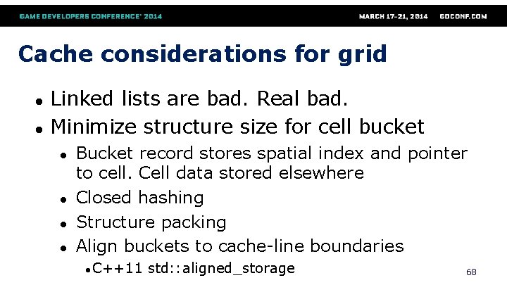
Cache considerations for grid ● ● Linked lists are bad. Real bad. Minimize structure size for cell bucket ● ● Bucket record stores spatial index and pointer to cell. Cell data stored elsewhere Closed hashing Structure packing Align buckets to cache-line boundaries ●C++11 std: : aligned_storage 68

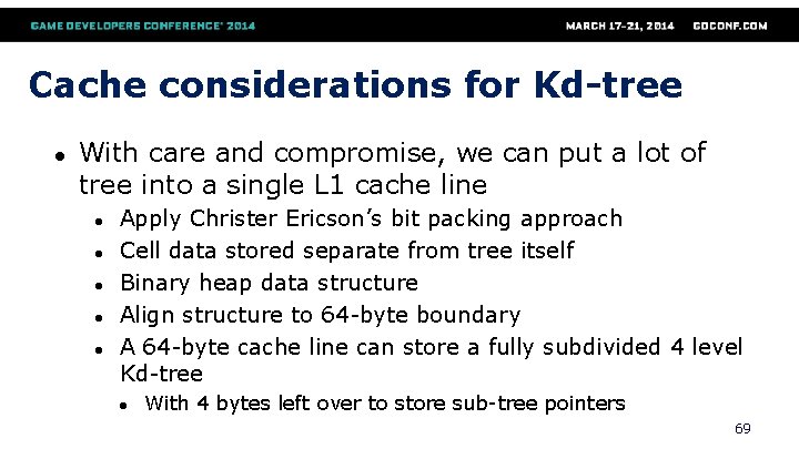
Cache considerations for Kd-tree ● With care and compromise, we can put a lot of tree into a single L 1 cache line ● ● ● Apply Christer Ericson’s bit packing approach Cell data stored separate from tree itself Binary heap data structure Align structure to 64 -byte boundary A 64 -byte cache line can store a fully subdivided 4 level Kd-tree ● With 4 bytes left over to store sub-tree pointers 69

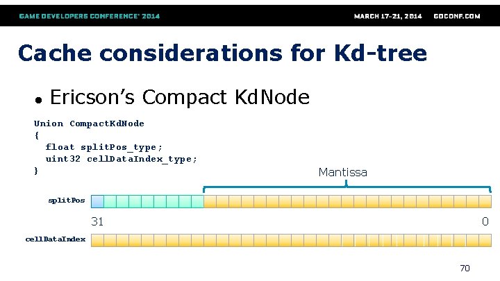
Cache considerations for Kd-tree ● Ericson’s Compact Kd. Node Union Compact. Kd. Node { float split. Pos_type; uint 32 cell. Data. Index_type; } Mantissa split. Pos 0 31 cell. Data. Index 70

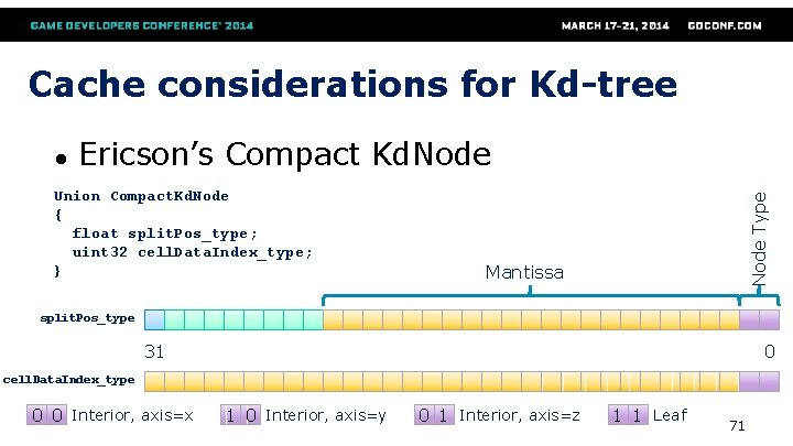
Cache considerations for Kd-tree Ericson’s Compact Kd. Node Union Compact. Kd. Node { float split. Pos_type; uint 32 cell. Data. Index_type; } Node Type ● Mantissa split. Pos_type 0 31 cell. Data. Index_type 0 0 Interior, axis=x 1 0 Interior, axis=y 0 1 Interior, axis=z 1 1 Leaf 71

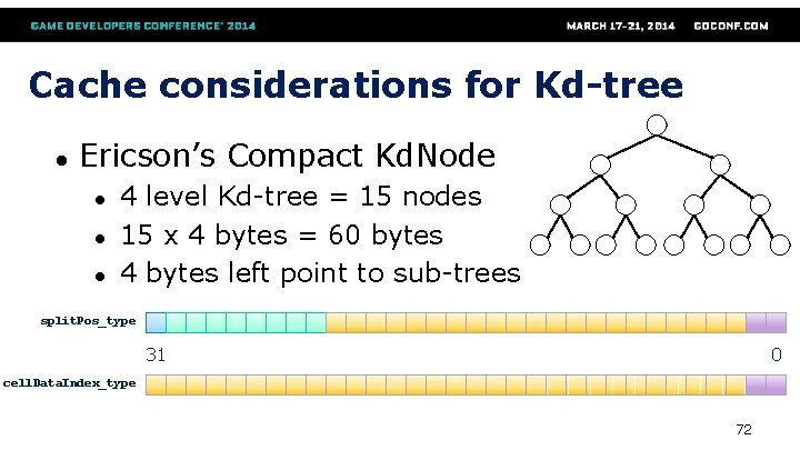
Cache considerations for Kd-tree ● Ericson’s Compact Kd. Node ● ● ● 4 level Kd-tree = 15 nodes 15 x 4 bytes = 60 bytes 4 bytes left point to sub-trees split. Pos_type 0 31 cell. Data. Index_type 72

References ● ● ● ● Ericson, Christer, Real-Time Collision Detection, Morgan Kaufmann Publishers/Elsevier, 2005 Hughes, John F. , et al. , Computer Graphics Principles and Practice, Third Edition, Addison-Wesley, 2014 Pharr, Matt, and Greg Humphreys, Physically-based Rendering, Morgan Kaufmann Publishers/Elsevier, 2004 Stoll, Gordon, “Ray Tracing Performance, ” SIGGRAPH 2005. Pascucci, Valerio, and Randall J. Frank, “Global Static Indexing for Real-time Exploration of Very Large Regular Grids, ” Supercomputing, ACM/IEEE 2001 Conference, 2001 http: //computinglife. wordpress. com/2008/11/20/why-do-hash-functions-use-primenumbers/ http: //www. bigprimes. net/ http: //www. 7 -cpu. com 73

Any Questions? Image is in the public domain. Painting date 1905. file source is http: //commons. wikimedia. org/wiki/File: Hooiberg_by_emile_claus. jpg 74