Spatial Relationship Global Spatial Autocorrelation measures Morans I
 • Global Spatial Autocorrelation measures • Moran’s I")
목차 • 공간 관계 (Spatial Relationship) • Global Spatial Autocorrelation measures • Moran’s I • Geary’s C • General G-statistic • Local Spatial Autocorrelation measures • LISA • Getis-Ord Gi* hot-spot analysis • Moran Scatterplot
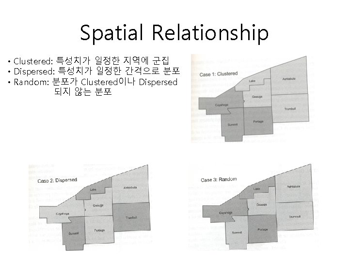

Spatial Autocorrelation • 특성치의 공간에 따른 연관성 degree of sameness of attribute values among areal units within their neighborhood 이웃한 polygon의 특성치가 유사 -> positive spatial autocorrelation의 정도? Strong or weak? 이웃한 polygon의 특성치가 규칙적으로 변화 -> negative spatial autocorrelation 이웃한 polygon의 특성치가 공간적으로 불규칙 분포 -> no spatial autocorrelation

Spatial Autocorrelation 정도 • Global Measure of spatial autocorrelation: Moran’s I, Geary’s Ratio C, G-statistic Assumption: spatial autocorrelation 이 주어진 지역에 대해 일정 -> spatial homogeneity • Local Measure of spatial autocorrelation: - LISA (Local Indicators of Spatial Autocorrelation) - Local version of G-statistic (Gi*) - Moran scatterplot
개념의 정량화 필요 Binary connectivity")
Spatial Weights Matrix • Spatial autocorrelation 계산 이전에 이웃 (neighborhood)개념의 정량화 필요 Binary connectivity matrix i polygon에 인접한 이웃의 j polygon i polygon에 인접하지 않는 이웃의 j polygon J=13 (# of joints) W=2 J=26

Spatial Weights Matrix Stochastic or Row-Standardized Weights Matrix
")
Spatial Weights Matrix Centroid Distance (inverse distance weighted)

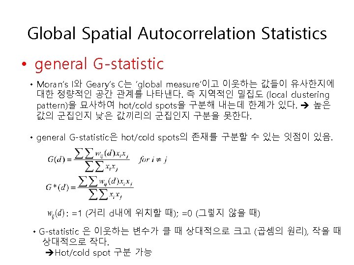
Global Spatial Autocorrelation Statistics • Moran’s I : 전체 평균, : Spatial weight matrix의 요소의 합, : 변수 수 • Moran’s I의 범위는 -1 (extremely negative spatial autocorrelation) 1 (extremely positive spatial autocorrelation) 사이 • spatial autocorrelation이 없는 경우 (random), Moran’s I의 기대값: 항상 음수이고 변수가 매우 클 때 음으로부터 0으로 수렴. 변수의 수가 적을 경우 음의 Moran’s I가 항상 negative spatial autocorrelation 을 의미하지 않는다. • Moran’s I의 계산에 있어 binary나 stochastic weight matrix가 주로 사용 • Moran’s I는 대상 변수 (xi)와 이웃하는 변수 (xj)의 전체평균으로부터의 편차의 곱 (공분산과 관계): High-High, Low-Low Positive spatial autocorrelation
")
• Moran’s I 계산 예제 (negative spatial autocorrelation? ? )
")
Significance test for Moran’s I • Moran’s I 기대값 (random distribution: no spatial autocorrelation) • Significance test (z-score) Variance of Moran’s I under the normality assumption Not significant random 패턴이 아니라고 말할 수 없다!

Global Spatial Autocorrelation Statistics • Geary’s Ratio, C • Geary’s C의 범위는 0 (extremely positive spatial autocorrelation) 2 (extremely negative spatial autocorrelation) 사이 • spatial autocorrelation이 없는 경우 (random), Geary’s C의 기대값: 1 • Geary’s C의 계산에 있어 binary나 stochastic weight matrix가 주로 사용 • Geary’s C는 대상 변수 (xi)와 이웃하는 변수 (xj)과의 차이의 제곱

• Geary’s C 계산 예제 Negative autocorrelation

• G-statistic 계산 예제

• G-statistic 계산 예제 Relatively large value: some types of clustering exist.
 Slightly")
Significance test for general G-statistic • General G-statistic 기대값 • Significance test (z-score) Slightly positive autocorrelation, but statistically not significant!
 • 어떤 지역들")
Local Spatial Autocorrelation Statistics • LISA (Local Indicator of Spatial Association) • 어떤 지역들 (subregions)에서 spatial autocorrelation이 다른 지역들에 비해 상대적으로 높을 때 global measure 사용은 적합치 않음. • 따라서 지역 마다 spatial autocorrelation를 나타내는 local measure가 필요 • LISA는 Moran’s I와 Geary’s C의 ‘local’ 버전으로 다음과 같이 정의된다. (Anselin, 1995) 이웃한 z-score의 비중에 따른 선형적 결합 z-score of xi • 일반적으로 wij는 stochastic (low-standardized matrix)
")
• LISA 계산 예제 (Local Moran’s I)

Significance test for Local Moran’s I • Local Moran’s I 기대값 • Significance test (z-score)

Local Spatial Autocorrelation Statistics • Local G-Statistic
 The Hot Spot Analysis tool calculates the")
Hot Spot Analysis: Getis-Ord Gi* (Spatial Statistics) The Hot Spot Analysis tool calculates the Getis-Ord Gi* statistic for each feature in a dataset. The resultant Z score tells you where features with either high or low values cluster spatially. This tool works by looking at each feature within the context of neighboring features. A feature with a high value is interesting, but may not be a statistically significant hot spot. To be a statistically significant hot spot, a feature will have a high value and be surrounded by other features with high values as well. The Gi* statistic returned for each feature in the dataset is a Z score. For statistically significant positive Z scores, the larger the Z score is, the more intense the clustering of high values (hot spot). For statistically significant negative Z scores, the smaller the Z score is, the more intense the clustering of low values (cold spot).
를 scatterplot")
Local Spatial Autocorrelation Statistics • Moran Scatterplot • Local Moran I ( )를 scatterplot 형태로 분포시켜 spatial autocorrelation의 지역적인 instability를 확인하는 데 매우 유용한 그림 x 축: standard variable( ), y축: spatial lag of that variable ( Low income with High income neighborhoods R 2=0. 87 Outlier Moran scatterplot의 기울기: Global Moran’s I High income with low income neighborhoods )

Local Spatial Autocorrelation Statistics • Moran Scatterplot Moran scatterplot의 기울기가 Global Moran’s I인 이유 일반적으로 scatterplot의 선형회귀식: y=a+bx where = Row-standardized

Local Spatial Autocorrelation Statistics • Moran Scatterplot example Moran’s I=0. 316 Positive spatial autocorrelation, but. .
- Slides: 25