Spatial Random Field Models Comparing CN Ratio among

Spatial Random Field Models – Comparing C/N Ratio among Tillage Treatments Vamsi Sundus Shawnalee

Purpose �“Data collected under different conditions (i. e. treatments) whether the conditions are different from each other and […] how the differences manifest themselves. ” �This data concerns soil.

The Setup �Soils are first chisel-plowed in the spring �Samples from 0 -2 inches were collected. �Measured N percentage (TN) �Measured C percentage (CN) �Calculated C/N, ratio between the two treatments. �Looking at the sample setup on 674, we see that it wasn’t randomly allocated. �We expect perhaps some spatial autocorrelation among the sample sites.

Simple calculations �Author: calculated simple pooled t-test: �p =. 809. �p > α �Thus no relation… �Doesn’t account for spatial autocorrelation among the 195 chisel-plow and 200 non-till strips. �Doesn’t convey the differences in the spatial structure of the treatments.

Analysis �They used SAS to obtain least squares + restricted maximum likelihood common nugget effect was fit. �Considerable variability of C/N ratios due to nugget effect. �Using “proc mixed” we get predictions of the C/N ratio.

Analysis (cont. ) �With proc mixed we assume that the C/N ratios are assumed to depend on the tillage treatments. �The SAS program is included in the section. Omitted since this is a class in R. �But, in the programming �Semivariogram – ensure both have same nugget effect.

Looking at the SAS Generated Output �Pg 677 -678 (SAS Output) �Looking at the curvy wavy thingy (surface plots) �We see one looks smoother and more predictable (no- tillage). This means greater spatial continuity (larger range). I. e. positive autocorrelations = stronger over same distance.

What does this mean? I know you’re lost. � At this point in the analysis: � There is no difference in the average C/N values in the study. [when sampling two months after installment of treatment. ] [pooled t-test] � There are differences in the spatial structure of the treatments [3 D plot]. � If we do a SSR (sum of squares reduction) we see that it’s extremely significant that a single spherical semivariogram cannot be used for bother semivariograms (Ha). � Using ordinary least squares we also find significance, but less so. �. 0001 versus. 00009 �. -3 -1 versus. -4 -9.

Next section

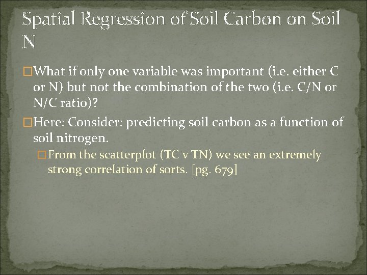
Spatial Regression of Soil Carbon on Soil N �What if only one variable was important (i. e. either C or N) but not the combination of the two (i. e. C/N or N/C ratio)? �Here: Consider: predicting soil carbon as a function of soil nitrogen. �From the scatterplot (TC v TN) we see an extremely strong correlation of sorts. [pg. 679]

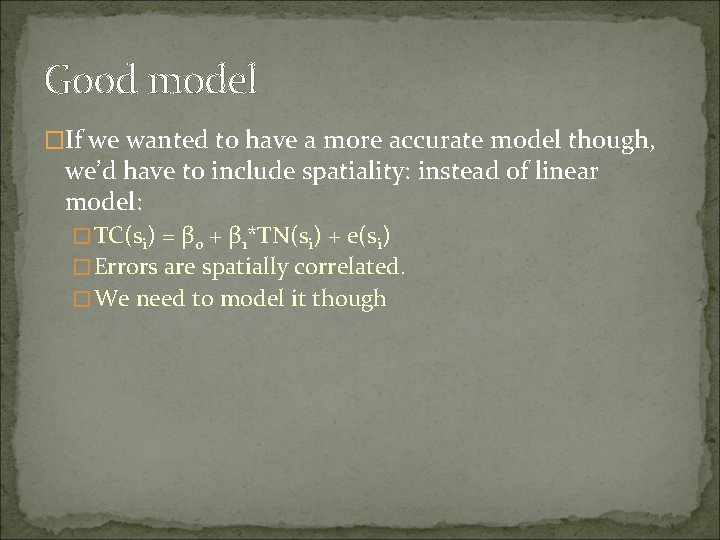
Good model �If we wanted to have a more accurate model though, we’d have to include spatiality: instead of linear model: �TC(si) = β 0 + β 1*TN(si) + e(si) �Errors are spatially correlated. �We need to model it though

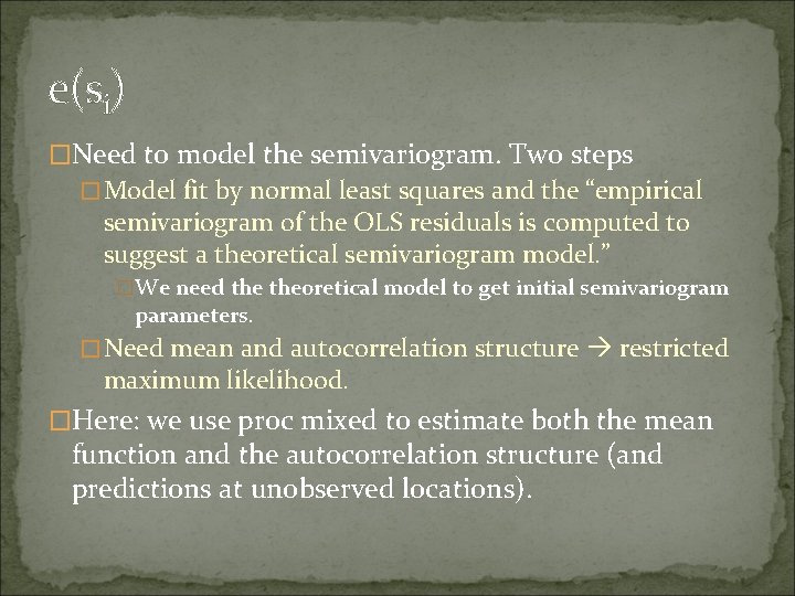
e(si) �Need to model the semivariogram. Two steps �Model fit by normal least squares and the “empirical semivariogram of the OLS residuals is computed to suggest a theoretical semivariogram model. ” �We need theoretical model to get initial semivariogram parameters. �Need mean and autocorrelation structure restricted maximum likelihood. �Here: we use proc mixed to estimate both the mean function and the autocorrelation structure (and predictions at unobserved locations).

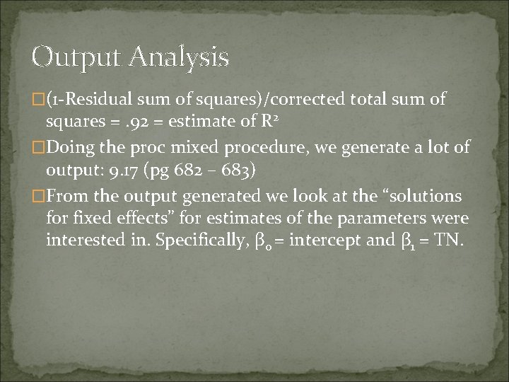
Output Analysis �(1 -Residual sum of squares)/corrected total sum of squares =. 92 = estimate of R 2 �Doing the proc mixed procedure, we generate a lot of output: 9. 17 (pg 682 – 683) �From the output generated we look at the “solutions for fixed effects” for estimates of the parameters were interested in. Specifically, β 0 = intercept and β 1 = TN.

What does this mean? �For every additional percent of N, we increase C by 11. 11 percentage points. �After playing a short game of “find the difference” on 9. 50, I see that they are nearly the same patterns. Wow…estimates of the expected value of TC and Predictions of TC are almost the same. Amazing! [pg 684]