Spatial Processing l Chris Rorden Spatial Registration l

Spatial Processing l Chris Rorden – Spatial Registration l l l – – – Motion correction Coregistration Normalization Interpolation Spatial Smoothing Advanced notes: l l l Spatial distortions of EPI scans Image intensity distortions Matrix mathematics 1

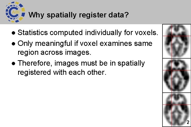
Why spatially register data? Statistics computed individually for voxels. l Only meaningful if voxel examines same region across images. l Therefore, images must be in spatially registered with each other. l 2

Spatial Registration l We use spatial registration to align images – – – Motion correction (realignment) adjusts for an individual’s head movements. Coregistration aligns two images of different modalities from the same individual. Normalization aligns images from different people. 3

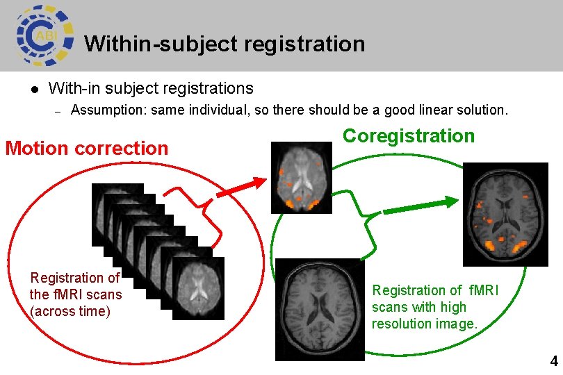
Within-subject registration l With-in subject registrations – Assumption: same individual, so there should be a good linear solution. Motion correction Registration of the f. MRI scans (across time) Coregistration Registration of f. MRI scans with high resolution image. 4

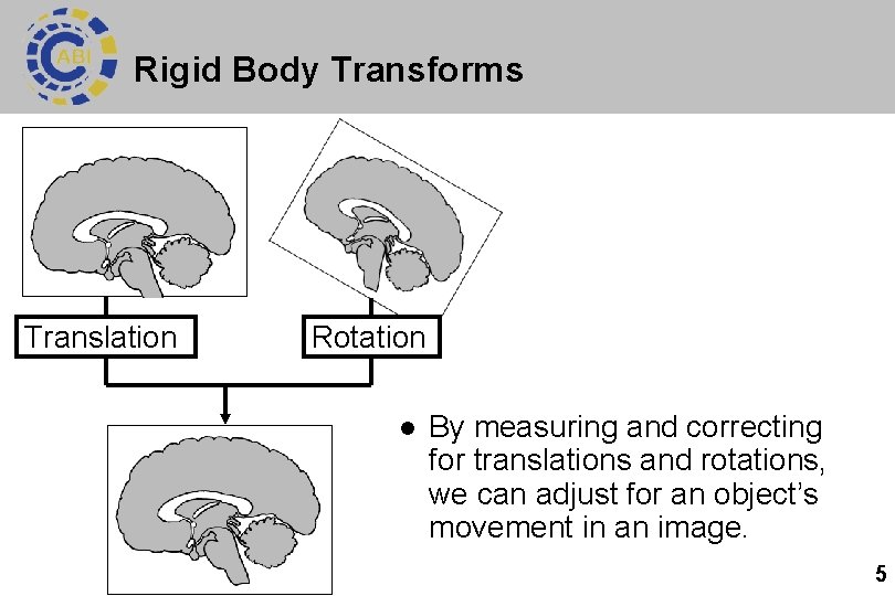
Rigid Body Transforms Translation Rotation l By measuring and correcting for translations and rotations, we can adjust for an object’s movement in an image. 5

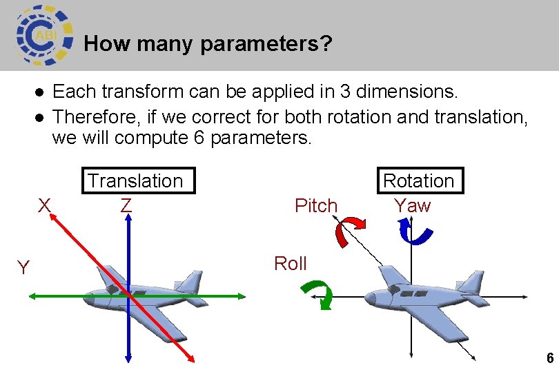
How many parameters? l l X Y Each transform can be applied in 3 dimensions. Therefore, if we correct for both rotation and translation, we will compute 6 parameters. Translation Z Pitch Rotation Yaw Roll 6

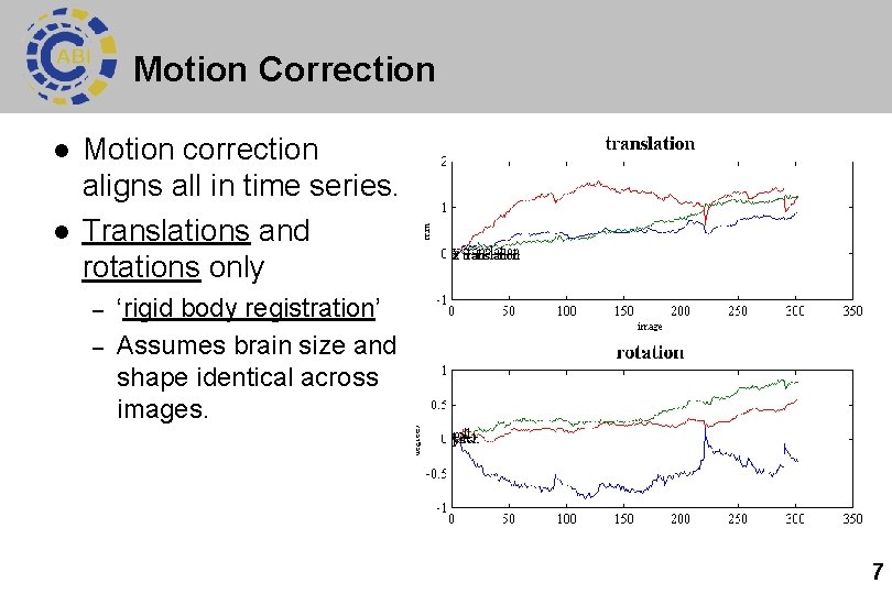
Motion Correction l l Motion correction aligns all in time series. Translations and rotations only – – ‘rigid body registration’ Assumes brain size and shape identical across images. 7

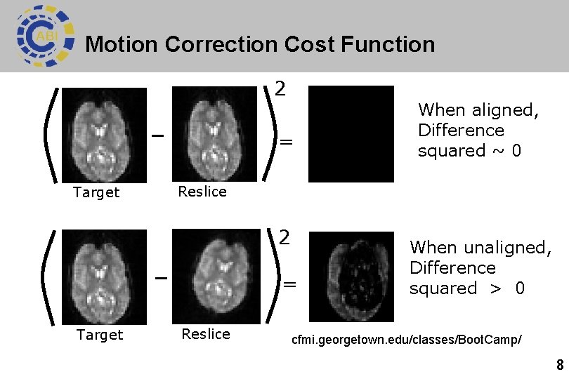
Motion Correction Cost Function 2 = Target Reslice 2 = Target When aligned, Difference squared ~ 0 Reslice When unaligned, Difference squared > 0 cfmi. georgetown. edu/classes/Boot. Camp/ 8

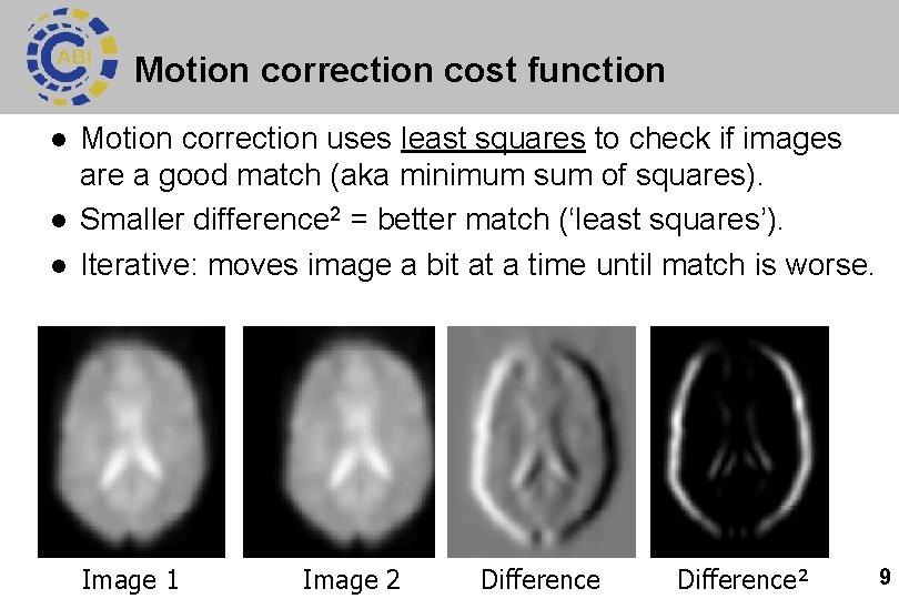
Motion correction cost function l l l Motion correction uses least squares to check if images are a good match (aka minimum sum of squares). Smaller difference 2 = better match (‘least squares’). Iterative: moves image a bit at a time until match is worse. Image 1 Image 2 Difference² 9

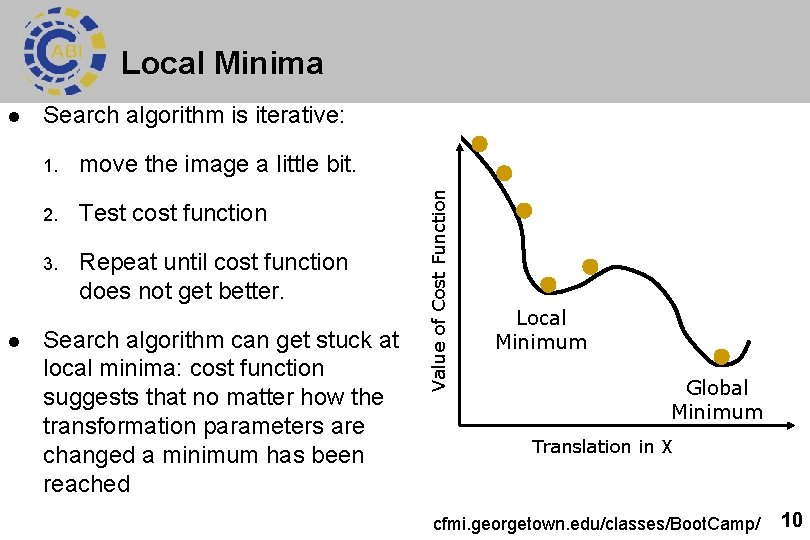
Local Minima l Search algorithm is iterative: 1. move the image a little bit. 2. Test cost function 3. Repeat until cost function does not get better. Search algorithm can get stuck at local minima: cost function suggests that no matter how the transformation parameters are changed a minimum has been reached Value of Cost Function l Local Minimum Global Minimum Translation in X cfmi. georgetown. edu/classes/Boot. Camp/ 10

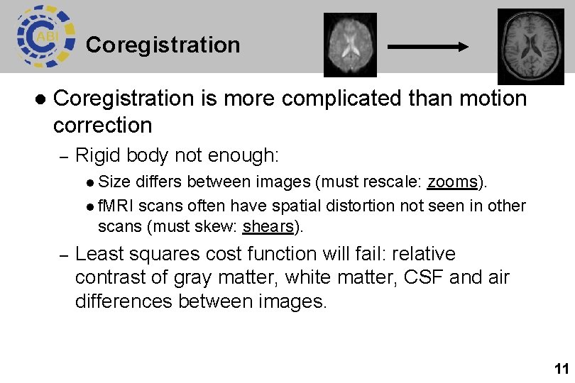
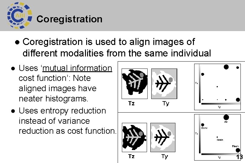
Coregistration l Coregistration is more complicated than motion correction – Rigid body not enough: l Size differs between images (must rescale: zooms). l f. MRI scans often have spatial distortion not seen in other scans (must skew: shears). – Least squares cost function will fail: relative contrast of gray matter, white matter, CSF and air differences between images. 11

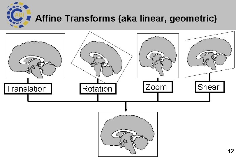
Affine Transforms (aka linear, geometric) Translation Rotation Zoom Shear 12

Coregistration l l l Coregistration is used to align images of different modalities from the same individual Uses ‘mutual information cost function’: Note aligned images have neater histograms. Uses entropy reduction instead of variance reduction as cost function. 13

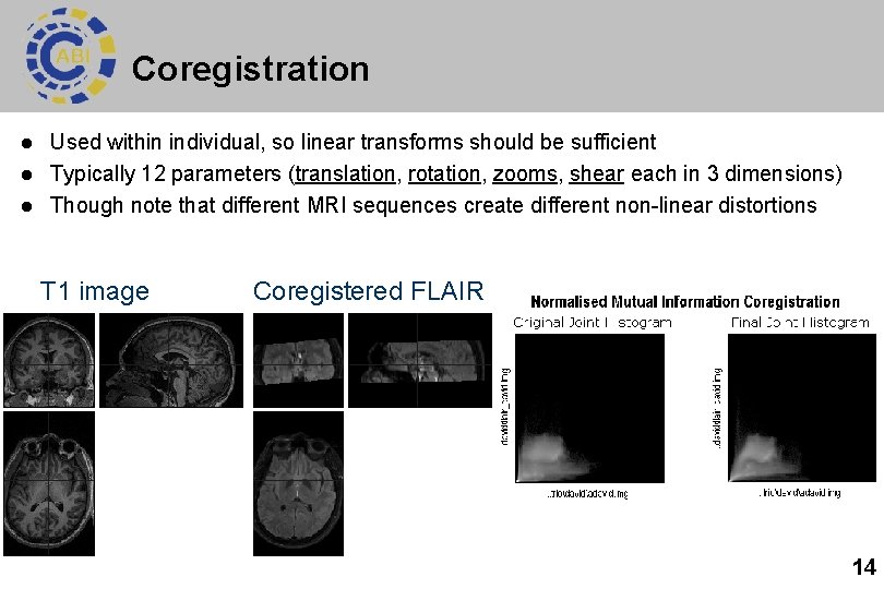
Coregistration l l l Used within individual, so linear transforms should be sufficient Typically 12 parameters (translation, rotation, zooms, shear each in 3 dimensions) Though note that different MRI sequences create different non-linear distortions T 1 image Coregistered FLAIR 14

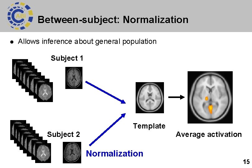
Between-subject: Normalization l Allows inference about general population Subject 1 Subject 2 Template Average activation Normalization 15

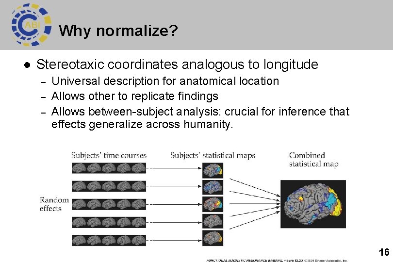
Why normalize? l Stereotaxic coordinates analogous to longitude – – – Universal description for anatomical location Allows other to replicate findings Allows between-subject analysis: crucial for inference that effects generalize across humanity. 16

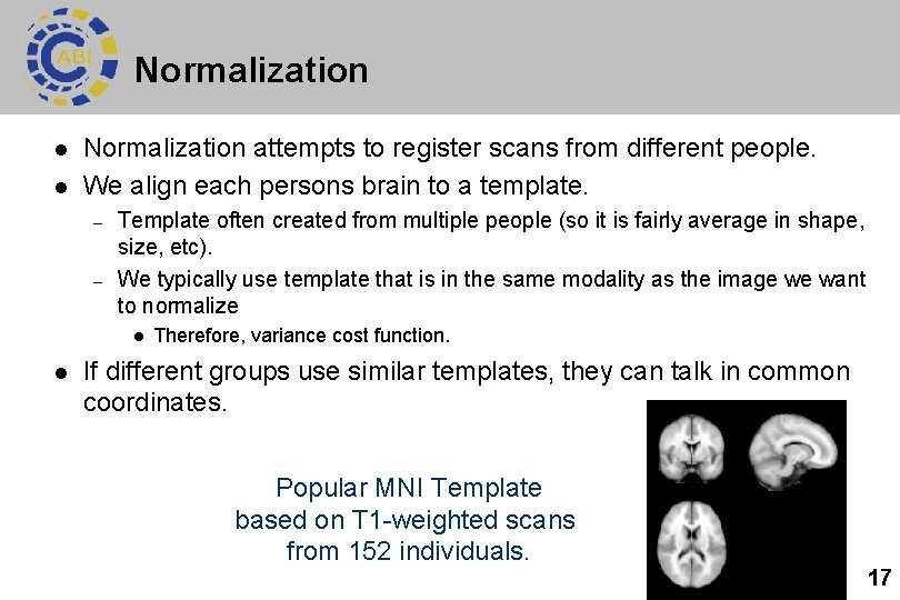
Normalization l l Normalization attempts to register scans from different people. We align each persons brain to a template. – – Template often created from multiple people (so it is fairly average in shape, size, etc). We typically use template that is in the same modality as the image we want to normalize l l Therefore, variance cost function. If different groups use similar templates, they can talk in common coordinates. Popular MNI Template based on T 1 -weighted scans from 152 individuals. 17

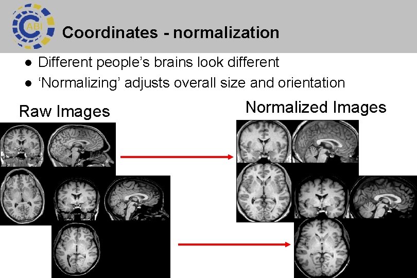
Coordinates - normalization l l Different people’s brains look different ‘Normalizing’ adjusts overall size and orientation Raw Images Normalized Images 18

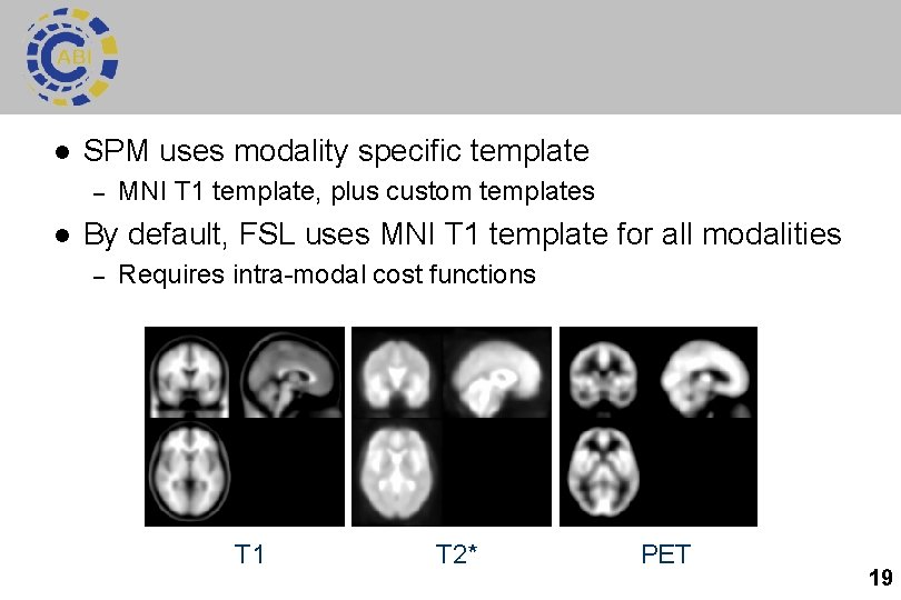
l SPM uses modality specific template – l MNI T 1 template, plus custom templates By default, FSL uses MNI T 1 template for all modalities – Requires intra-modal cost functions T 1 T 2* PET 19

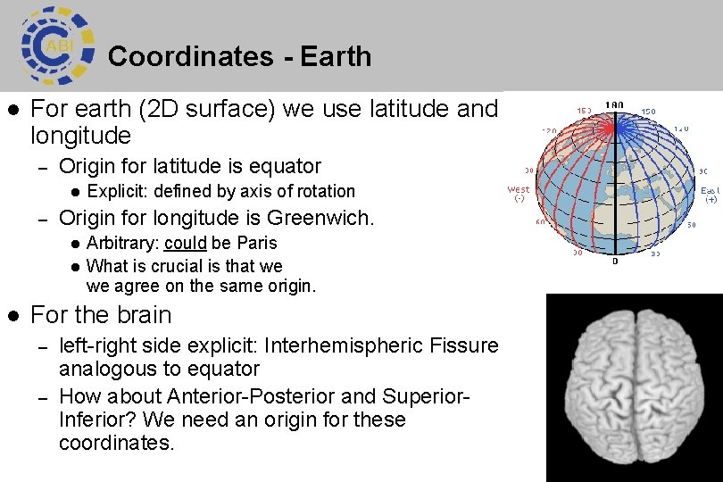
Coordinates - Earth l For earth (2 D surface) we use latitude and longitude – Origin for latitude is equator l – Origin for longitude is Greenwich. l l l Explicit: defined by axis of rotation Arbitrary: could be Paris What is crucial is that we we agree on the same origin. For the brain – – left-right side explicit: Interhemispheric Fissure analogous to equator How about Anterior-Posterior and Superior. Inferior? We need an origin for these coordinates. 20

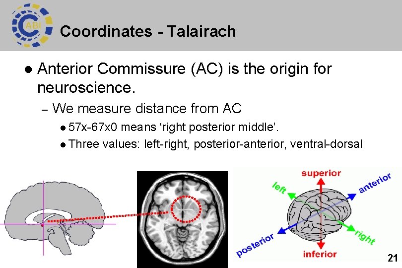
Coordinates - Talairach l Anterior Commissure (AC) is the origin for neuroscience. – We measure distance from AC l 57 x-67 x 0 means ‘right posterior middle’. l Three values: left-right, posterior-anterior, ventral-dorsal 21

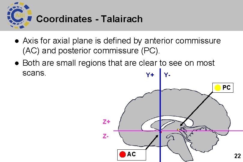
Coordinates - Talairach l l Axis for axial plane is defined by anterior commissure (AC) and posterior commissure (PC). Both are small regions that are clear to see on most scans. Y+ Y PC Z+ Z AC 22

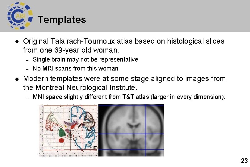
Templates l Original Talairach-Tournoux atlas based on histological slices from one 69 -year old woman. – – l Single brain may not be representative No MRI scans from this woman Modern templates were at some stage aligned to images from the Montreal Neurological Institute. – MNI space slightly different from T&T atlas (larger in every dimension). 23

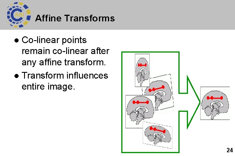
Affine Transforms Co-linear points remain co-linear after any affine transform. l Transform influences entire image. l 24

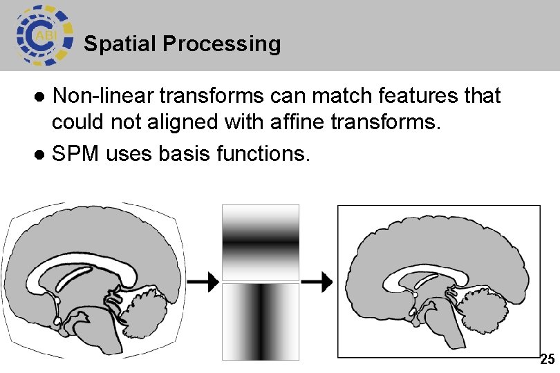
Spatial Processing Non-linear transforms can match features that could not aligned with affine transforms. l SPM uses basis functions. l 25

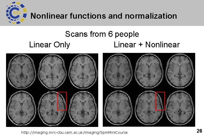
Nonlinear functions and normalization Scans from 6 people Linear Only Linear + Nonlinear http: //imaging. mrc-cbu. cam. ac. uk/imaging/Spm. Mini. Course 26

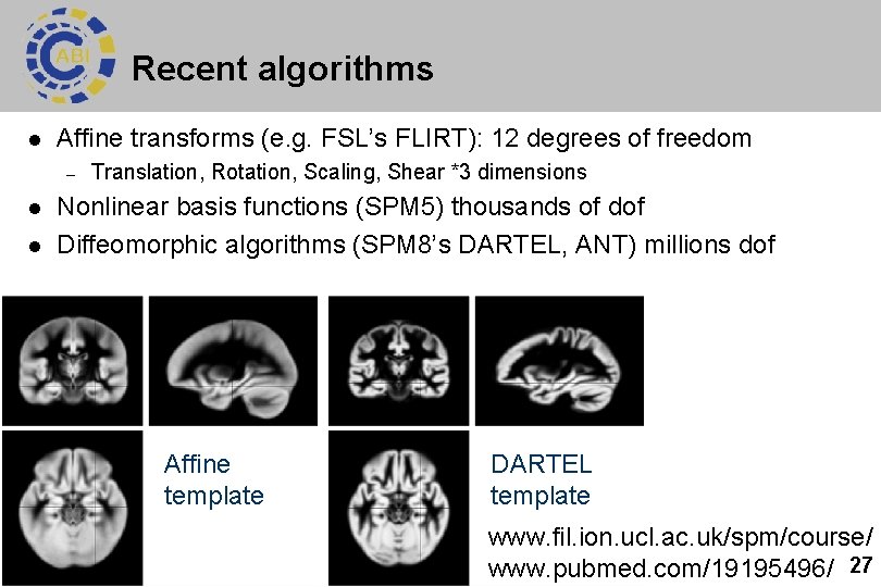
Recent algorithms l Affine transforms (e. g. FSL’s FLIRT): 12 degrees of freedom – l l Translation, Rotation, Scaling, Shear *3 dimensions Nonlinear basis functions (SPM 5) thousands of dof Diffeomorphic algorithms (SPM 8’s DARTEL, ANT) millions dof Affine template DARTEL template www. fil. ion. ucl. ac. uk/spm/course/ www. pubmed. com/19195496/ 27

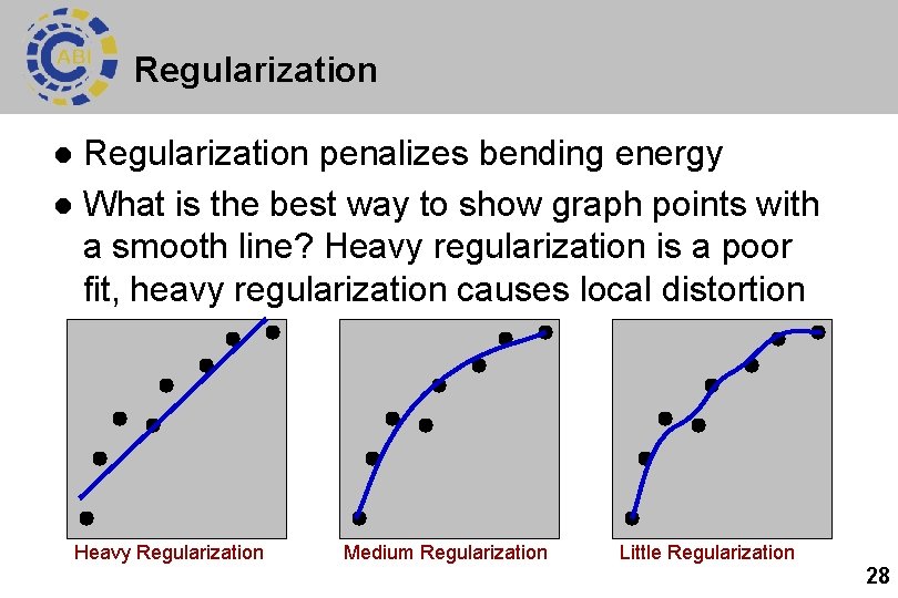
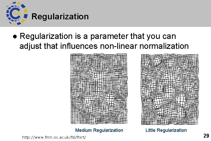
Regularization penalizes bending energy l What is the best way to show graph points with a smooth line? Heavy regularization is a poor fit, heavy regularization causes local distortion l Heavy Regularization Medium Regularization Little Regularization 28

Regularization l Regularization is a parameter that you can adjust that influences non-linear normalization Medium Regularization http: //www. fmri. ox. ac. uk/fsl/fnirt/ Little Regularization 29

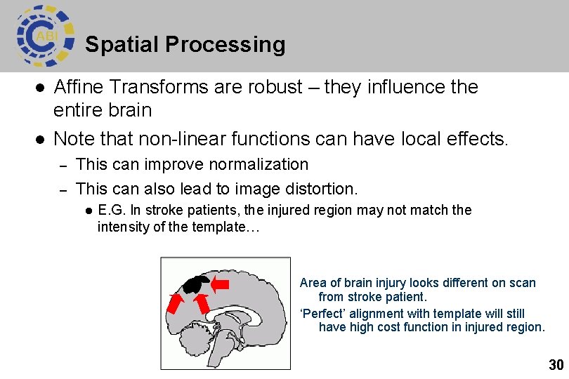
Spatial Processing l l Affine Transforms are robust – they influence the entire brain Note that non-linear functions can have local effects. – – This can improve normalization This can also lead to image distortion. l E. G. In stroke patients, the injured region may not match the intensity of the template… Area of brain injury looks different on scan from stroke patient. ‘Perfect’ alignment with template will still have high cost function in injured region. 30

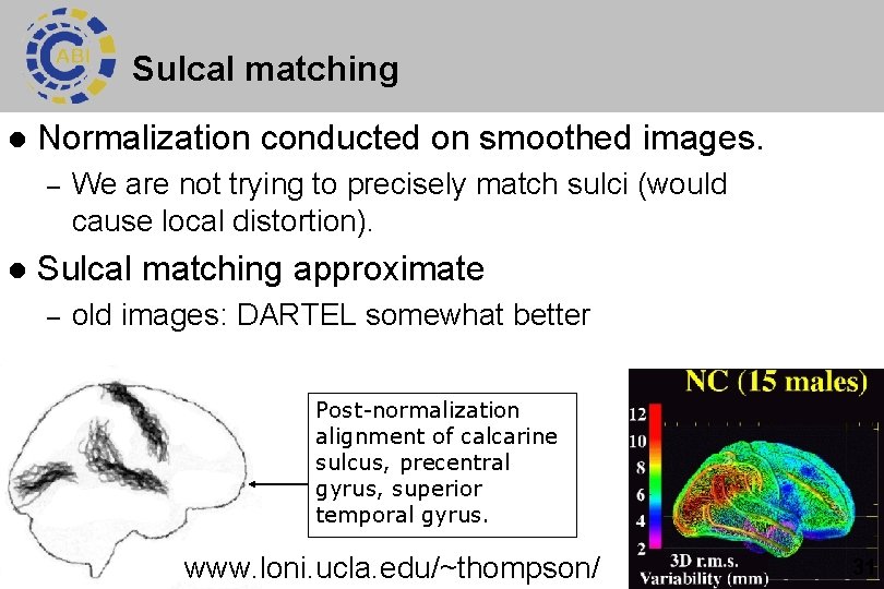
Sulcal matching l Normalization conducted on smoothed images. – l We are not trying to precisely match sulci (would cause local distortion). Sulcal matching approximate – old images: DARTEL somewhat better Post-normalization alignment of calcarine sulcus, precentral gyrus, superior temporal gyrus. www. loni. ucla. edu/~thompson/ 31

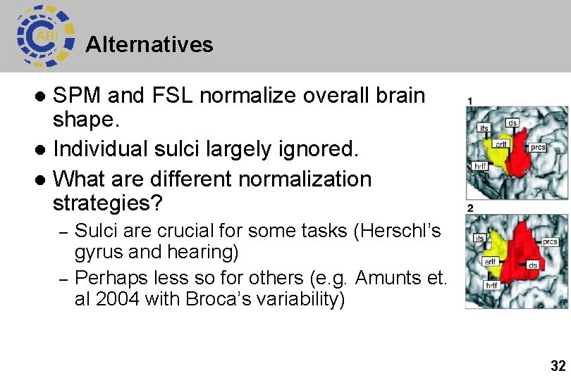
Alternatives SPM and FSL normalize overall brain shape. l Individual sulci largely ignored. l What are different normalization strategies? l – – Sulci are crucial for some tasks (Herschl’s gyrus and hearing) Perhaps less so for others (e. g. Amunts et. al 2004 with Broca’s variability) 32

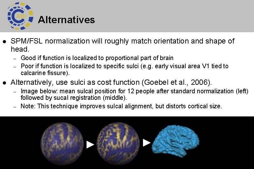
Alternatives l SPM/FSL normalization will roughly match orientation and shape of head. – – l Good if function is localized to proportional part of brain Poor if function is localized to specific sulci (e. g. early visual area V 1 tied to calcarine fissure). Alternatively, use sulci as cost function (Goebel et al. , 2006). – – Image below: mean sulcal position for 12 people after standard normalization (left) followed by sucal registration (middle). Note: This technique improves sulcal alignment, but distorts cortical size. 33

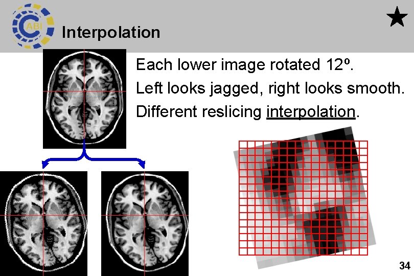
Interpolation Each lower image rotated 12º. Left looks jagged, right looks smooth. Different reslicing interpolation. 34

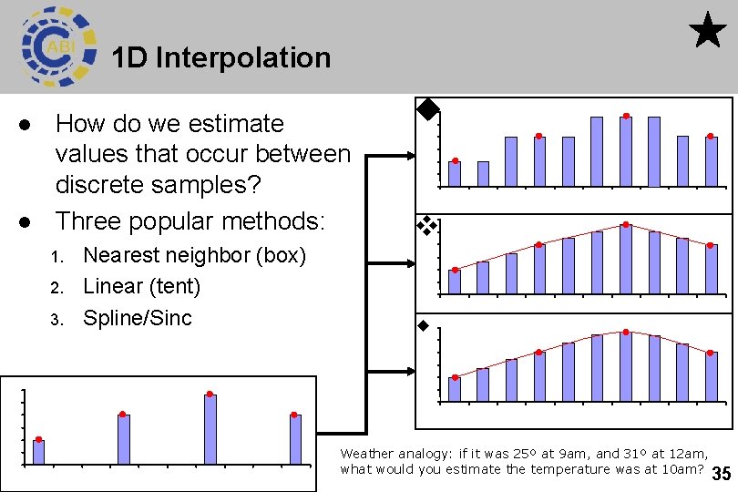
1 D Interpolation l l How do we estimate values that occur between discrete samples? Three popular methods: 1. 2. 3. Nearest neighbor (box) Linear (tent) Spline/Sinc Weather analogy: if it was 25º at 9 am, and 31º at 12 am, what would you estimate the temperature was at 10 am? 35

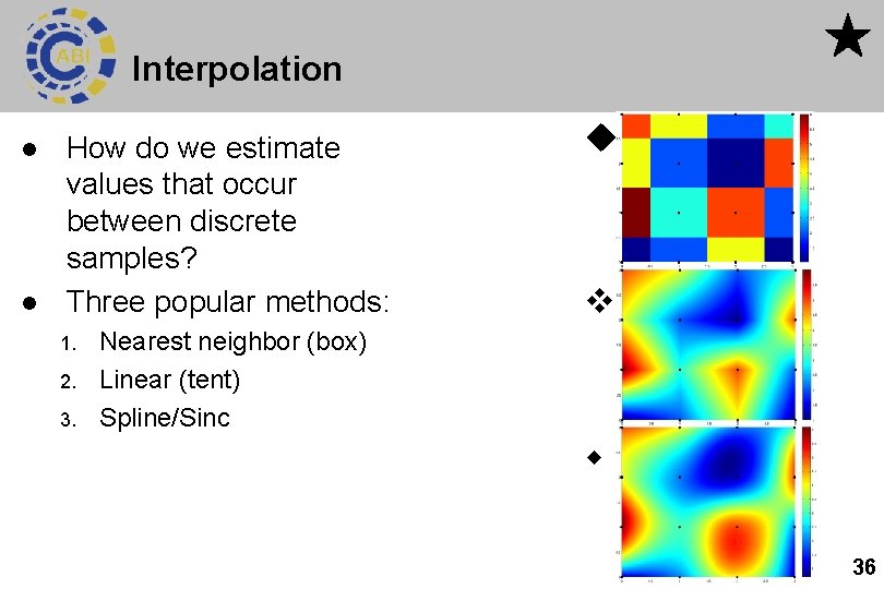
Interpolation l l How do we estimate values that occur between discrete samples? Three popular methods: 1. 2. 3. Nearest neighbor (box) Linear (tent) Spline/Sinc 36

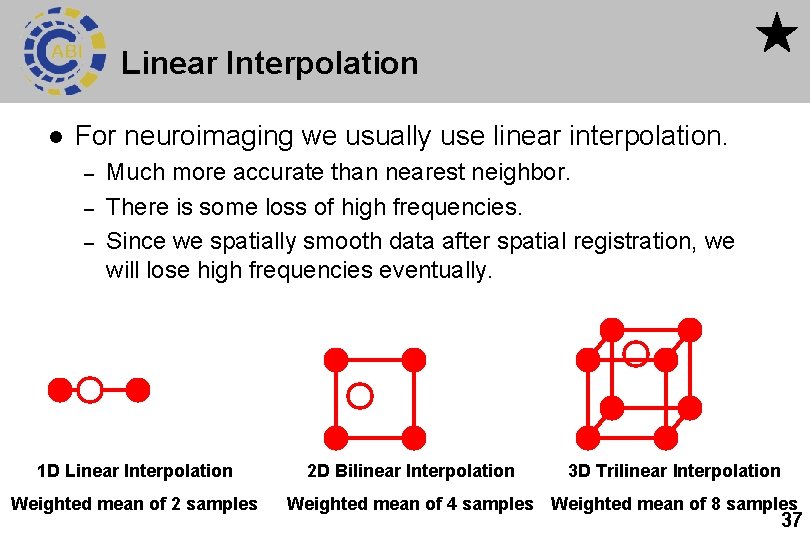
Linear Interpolation l For neuroimaging we usually use linear interpolation. – – – Much more accurate than nearest neighbor. There is some loss of high frequencies. Since we spatially smooth data after spatial registration, we will lose high frequencies eventually. 1 D Linear Interpolation Weighted mean of 2 samples 2 D Bilinear Interpolation 3 D Trilinear Interpolation Weighted mean of 4 samples Weighted mean of 8 samples 37

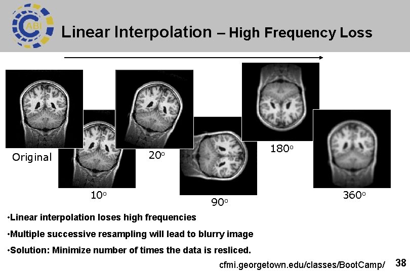
Linear Interpolation – High Frequency Loss 180 o 20 o Original 10 o 90 o 360 o • Linear interpolation loses high frequencies • Multiple successive resampling will lead to blurry image • Solution: Minimize number of times the data is resliced. cfmi. georgetown. edu/classes/Boot. Camp/ 38

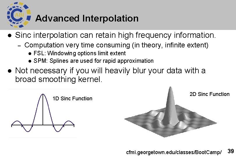
Advanced Interpolation l Sinc interpolation can retain high frequency information. – Computation very time consuming (in theory, infinite extent) l l l FSL: Windowing options limit extent SPM: Splines are used for rapid approximation Not necessary if you will heavily blur your data with a broad smoothing kernel. 1 D Sinc Function 2 D Sinc Function cfmi. georgetown. edu/classes/Boot. Camp/ 39

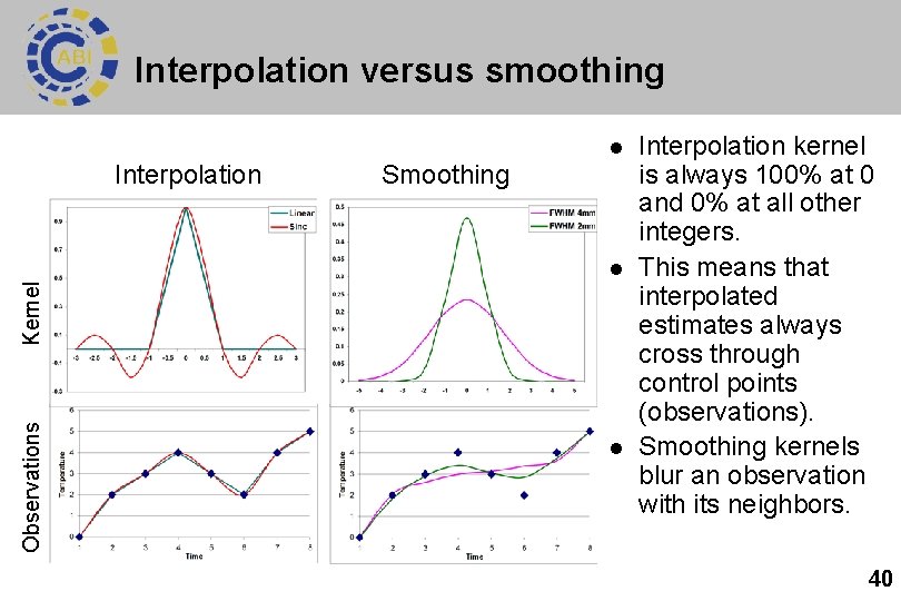
Interpolation versus smoothing l Interpolation Smoothing Observations Kernel l l Interpolation kernel is always 100% at 0 and 0% at all other integers. This means that interpolated estimates always cross through control points (observations). Smoothing kernels blur an observation with its neighbors. 40

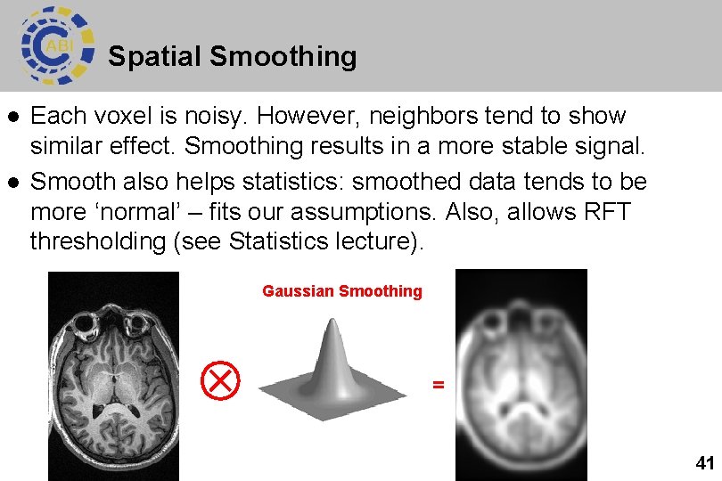
Spatial Smoothing l l Each voxel is noisy. However, neighbors tend to show similar effect. Smoothing results in a more stable signal. Smooth also helps statistics: smoothed data tends to be more ‘normal’ – fits our assumptions. Also, allows RFT thresholding (see Statistics lecture). Gaussian Smoothing = 41

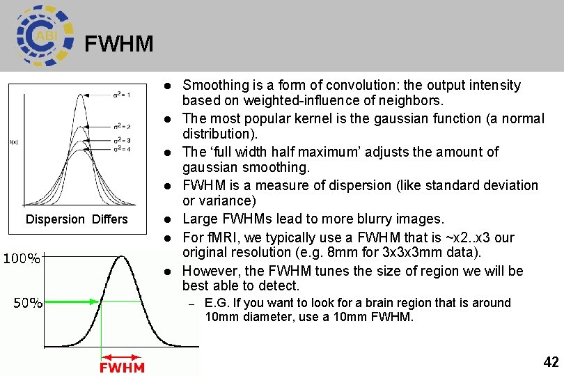
FWHM l l Dispersion Differs l l l Smoothing is a form of convolution: the output intensity based on weighted-influence of neighbors. The most popular kernel is the gaussian function (a normal distribution). The ‘full width half maximum’ adjusts the amount of gaussian smoothing. FWHM is a measure of dispersion (like standard deviation or variance) Large FWHMs lead to more blurry images. For f. MRI, we typically use a FWHM that is ~x 2. . x 3 our original resolution (e. g. 8 mm for 3 x 3 x 3 mm data). However, the FWHM tunes the size of region we will be best able to detect. – E. G. If you want to look for a brain region that is around 10 mm diameter, use a 10 mm FWHM. 42

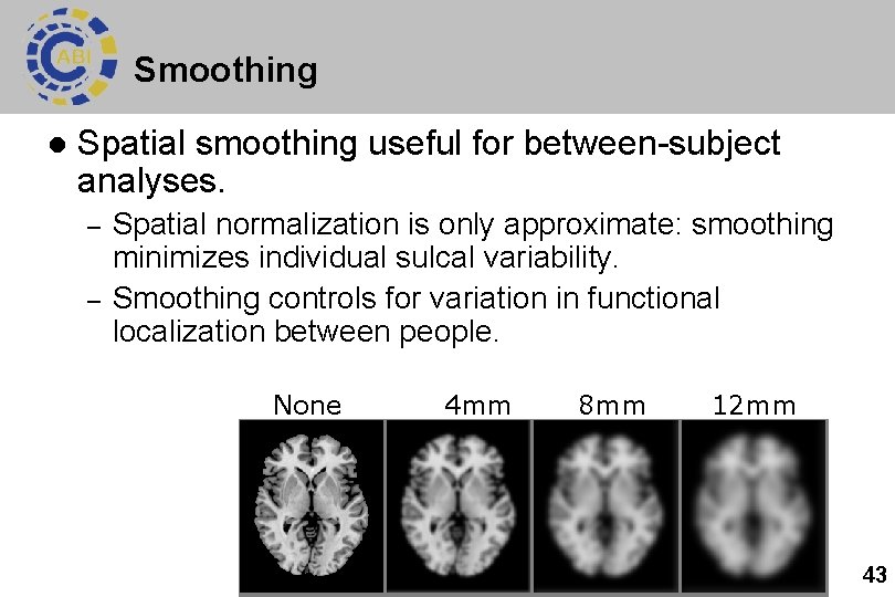
Smoothing l Spatial smoothing useful for between-subject analyses. – – Spatial normalization is only approximate: smoothing minimizes individual sulcal variability. Smoothing controls for variation in functional localization between people. None 4 mm 8 mm 12 mm 43

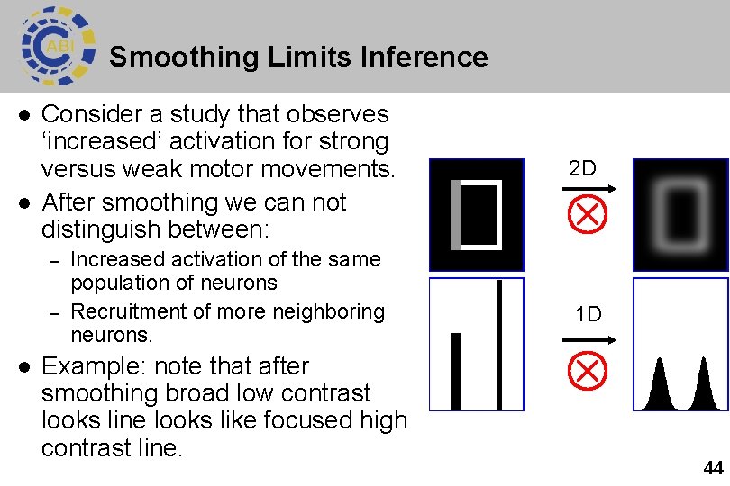
Smoothing Limits Inference l l Consider a study that observes ‘increased’ activation for strong versus weak motor movements. After smoothing we can not distinguish between: – – l Increased activation of the same population of neurons Recruitment of more neighboring neurons. Example: note that after smoothing broad low contrast looks line looks like focused high contrast line. 2 D 1 D 44

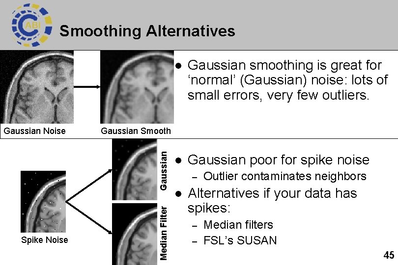
Smoothing Alternatives Median Filter Spike Noise Gaussian smoothing is great for ‘normal’ (Gaussian) noise: lots of small errors, very few outliers. l Gaussian poor for spike noise Gaussian Smooth Gaussian Noise l – l Outlier contaminates neighbors Alternatives if your data has spikes: – – Median filters FSL’s SUSAN 45

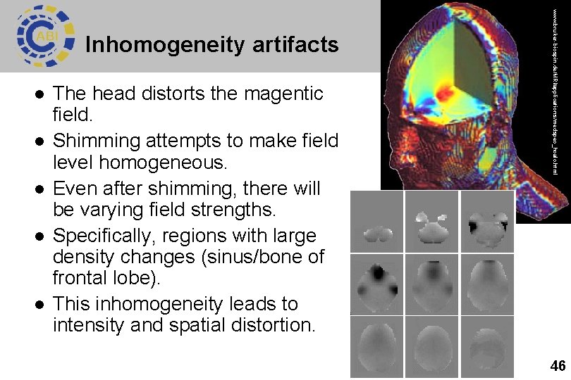
l l l The head distorts the magentic field. Shimming attempts to make field level homogeneous. Even after shimming, there will be varying field strengths. Specifically, regions with large density changes (sinus/bone of frontal lobe). This inhomogeneity leads to intensity and spatial distortion. www. bruker-biospin. de/MRI/applications/medspec_hcalc. html Inhomogeneity artifacts 46

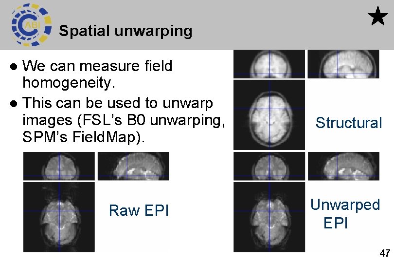
Spatial unwarping We can measure field homogeneity. l This can be used to unwarp images (FSL’s B 0 unwarping, SPM’s Field. Map). l Raw EPI Structural Unwarped EPI 47

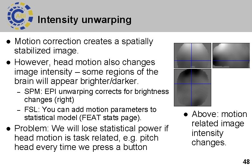
Intensity unwarping l l Motion correction creates a spatially stabilized image. However, head motion also changes image intensity – some regions of the brain will appear brighter/darker. – – l SPM: EPI unwarping corrects for brightness changes (right) FSL: You can add motion parameters to statistical model (FEAT stats page). Problem: We will lose statistical power if head motion is task related, e. g. pitch head every time we press a button l Above: motion related image intensity changes. 48

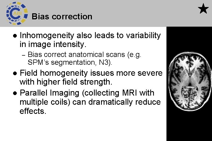
Bias correction l Inhomogeneity also leads to variability in image intensity. – Bias correct anatomical scans (e. g. SPM’s segmentation, N 3). Field homogeneity issues more severe with higher field strength. l Parallel Imaging (collecting MRI with multiple coils) can dramatically reduce effects. l 49

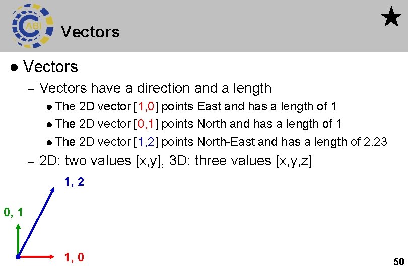
Vectors l Vectors – Vectors have a direction and a length l The 2 D vector [1, 0] points East and has a length of 1 l The 2 D vector [0, 1] points North and has a length of 1 l The 2 D vector [1, 2] points North-East and has a length of 2. 23 – 2 D: two values [x, y], 3 D: three values [x, y, z] 1, 2 0, 1 1, 0 50

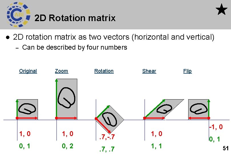
2 D Rotation matrix l 2 D rotation matrix as two vectors (horizontal and vertical) – Can be described by four numbers Original Zoom Rotation Shear 1, 0 . 7, -. 7 1, 0 0, 1 0, 2 . 7, . 7 1, 1 Flip -1, 0 0, 1 51

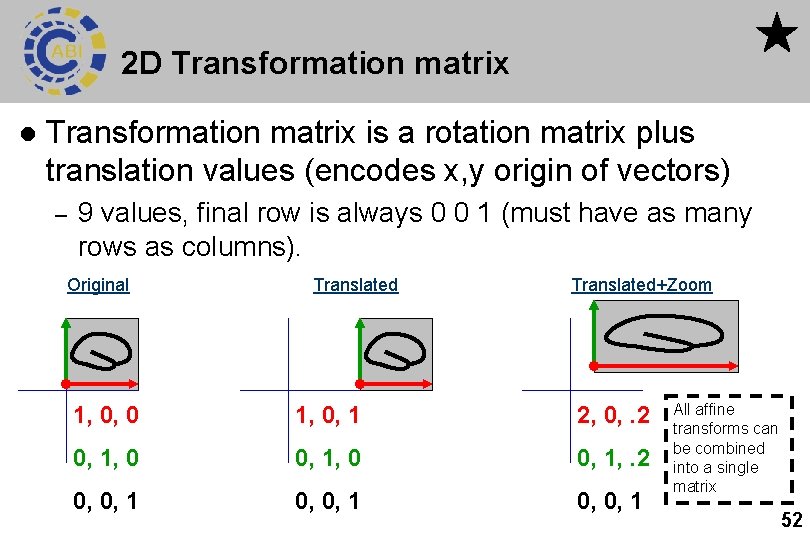
2 D Transformation matrix l Transformation matrix is a rotation matrix plus translation values (encodes x, y origin of vectors) – 9 values, final row is always 0 0 1 (must have as many rows as columns). Original Translated+Zoom 1, 0, 0 1, 0, 1 2, 0, . 2 0, 1, 0 0, 1, . 2 0, 0, 1 All affine transforms can be combined into a single matrix 52

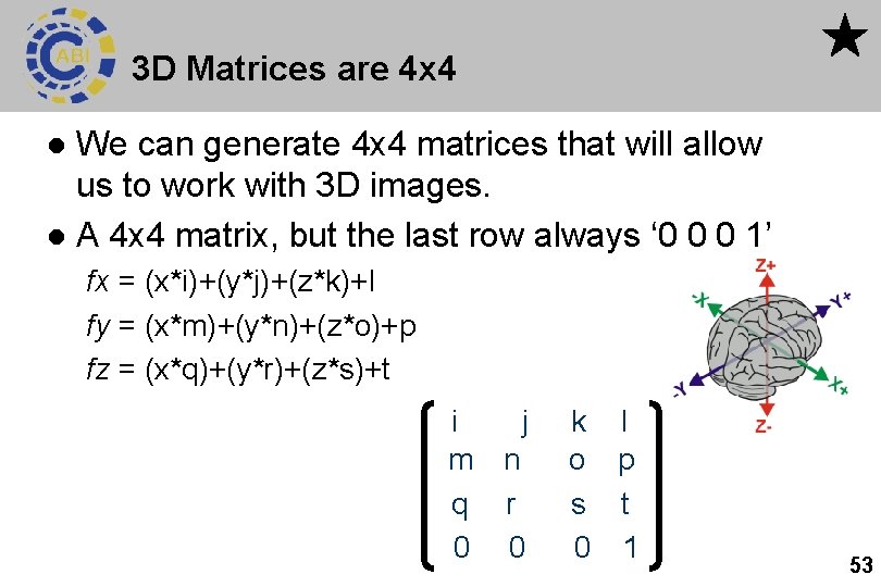
3 D Matrices are 4 x 4 We can generate 4 x 4 matrices that will allow us to work with 3 D images. l A 4 x 4 matrix, but the last row always ‘ 0 0 0 1’ l fx = (x*i)+(y*j)+(z*k)+l fy = (x*m)+(y*n)+(z*o)+p fz = (x*q)+(y*r)+(z*s)+t i j m n q r 0 0 k l o p s t 0 1 53

Matrices and 3 D space l 3 D matrices work just like 2 D matrices – – – The identity matrix still has 1’s along the diagonal Translations are the values in the final column (constants) Zooms are done by scaling values of a row. Shears are values added to the relevant orthogonal value Rotations use sine/cosine in dimensions of plane. Our twelve numbers can store all of the possible rotations, shears, translations and scaling. l Simply multiply previous matrix with our transform (order crucial). 54