Spatial Preprocessing Ged Ridgway FMRIBFIL With thanks to

Spatial Preprocessing Ged Ridgway, FMRIB/FIL With thanks to John Ashburner and the FIL Methods Group

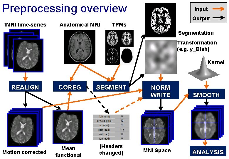
Preprocessing overview Input Output f. MRI time-series Anatomical MRI TPMs Segmentation Transformation (e. g. y_Blah) Kernel REALIGN Motion corrected COREG Mean functional SEGMENT (Headers changed) NORM WRITE MNI Space SMOOTH ANALYSIS

Reorientation and registration demo • Now to SPM… • … for a more conventional slide-based talk, please see the video (with accompanying slides available) at www. fil. ion. ucl. ac. uk/spm/course/video/

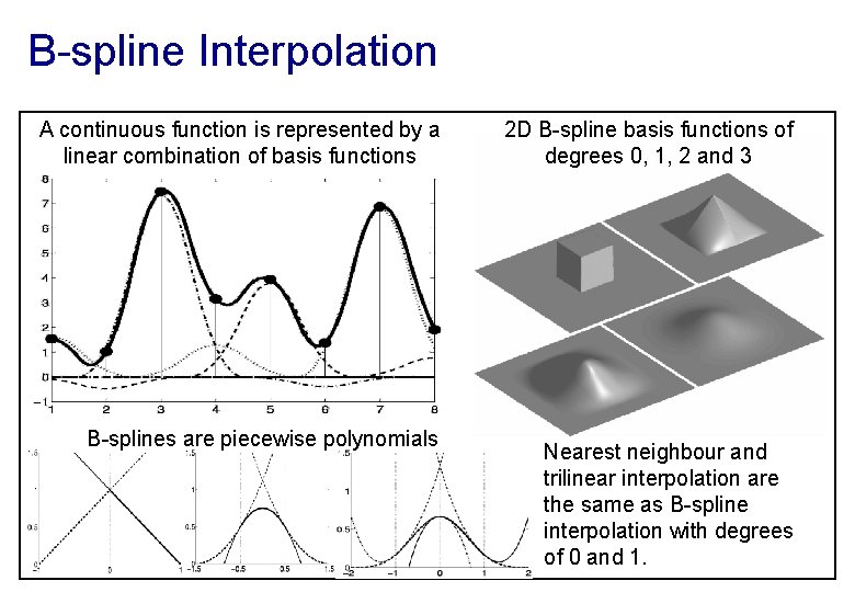
B-spline Interpolation A continuous function is represented by a linear combination of basis functions B-splines are piecewise polynomials 2 D B-spline basis functions of degrees 0, 1, 2 and 3 Nearest neighbour and trilinear interpolation are the same as B-spline interpolation with degrees of 0 and 1.

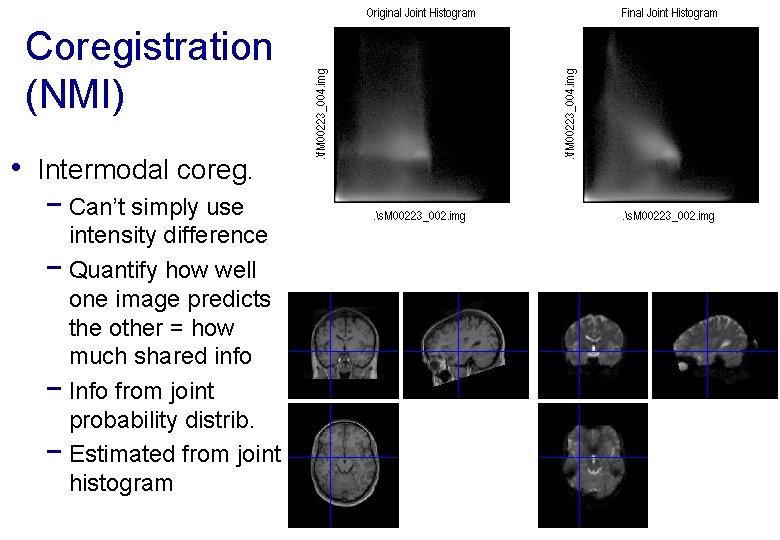
Coregistration (NMI) • Intermodal coreg. − Can’t simply use intensity difference − Quantify how well one image predicts the other = how much shared info − Info from joint probability distrib. − Estimated from joint histogram

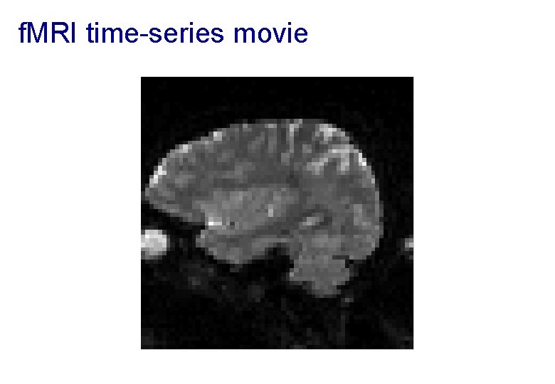
f. MRI time-series movie

Motion in f. MRI • Is important! − − Increases residual variance and reduces sensitivity Data may get completely lost with sudden movements Movements may be correlated with the task Try to minimise movement (don’t scan for too long!) • Motion correction using realignment − Each volume rigidly registered to reference − Least squares objective function • Realigned images must be resliced for analysis − Not necessary if they will be normalised anyway

Residual Errors from aligned f. MRI • Slices are not acquired simultaneously − rapid movements not accounted for by rigid body model • Image artefacts may not move according to a rigid body model − image distortion, image dropout, Nyquist ghost • Gaps between slices can cause aliasing artefacts • Re-sampling can introduce interpolation errors − Though higher degree spline interpolation mitigates • Functions of the estimated motion parameters can be modelled as confounds in subsequent analyses

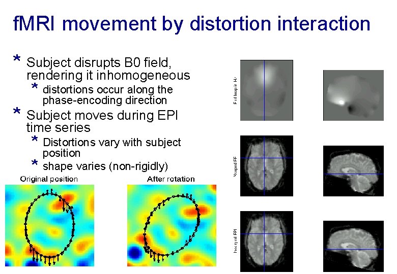
f. MRI movement by distortion interaction * Subject disrupts B 0 field, rendering it inhomogeneous * distortions occur along the phase-encoding direction * Subject moves during EPI time series * Distortions vary with subject * position shape varies (non-rigidly)

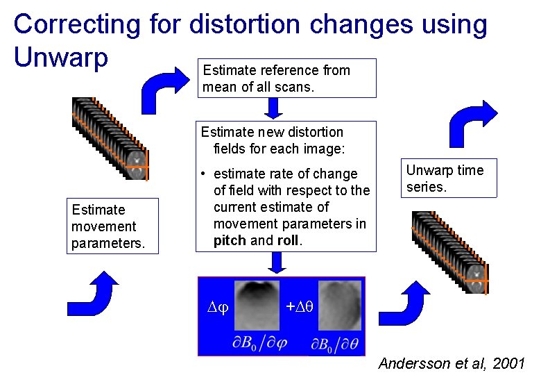
Correcting for distortion changes using Unwarp Estimate reference from mean of all scans. Estimate new distortion fields for each image: Estimate movement parameters. • estimate rate of change of field with respect to the current estimate of movement parameters in pitch and roll. Unwarp time series. + Andersson et al, 2001

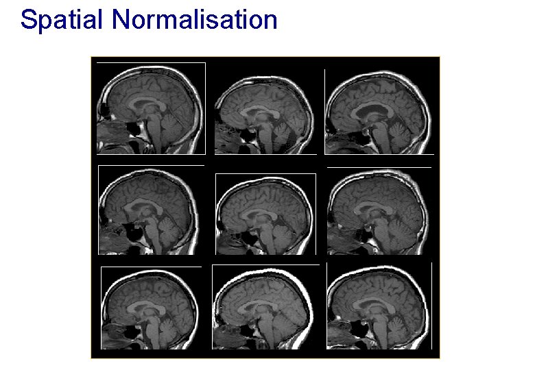
Spatial Normalisation

Spatial Normalisation - Reasons • Inter-subject averaging − Increase sensitivity with more subjects • Fixed-effects analysis − Extrapolate findings to the population as a whole • Mixed-effects analysis • Make results from different studies comparable by aligning them to standard space − e. g. The T&T convention, using the MNI template

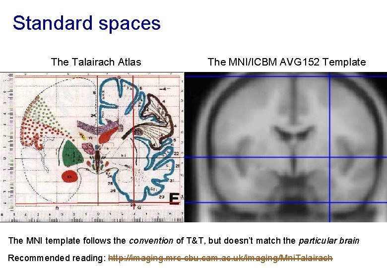
Standard spaces The Talairach Atlas The MNI/ICBM AVG 152 Template The MNI template follows the convention of T&T, but doesn’t match the particular brain Recommended reading: http: //imaging. mrc-cbu. cam. ac. uk/imaging/Mni. Talairach

Normalisation via unified segmentation • MRI imperfections make normalisation harder − Noise, artefacts, partial volume effect − Intensity inhomogeneity or “bias” field − Differences between sequences • Normalising segmented tissue maps should be more • robust and precise than using the original images. . . … Tissue segmentation benefits from spatially-aligned prior tissue probability maps (from other segmentations) • This circularity motivates simultaneous segmentation and normalisation in a unified model

Summary of the unified model • SPM 12 implements a generative model − Principled Bayesian probabilistic formulation • Gaussian mixture model segmentation with deformable tissue probability maps (priors) − The inverse of the transformation that aligns the TPMs can be used to normalise the original image • Bias correction is included within the model

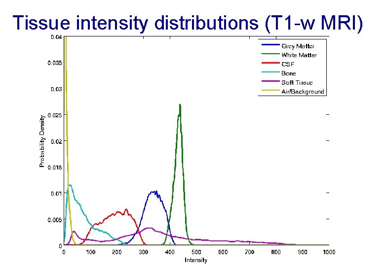
Tissue intensity distributions (T 1 -w MRI)

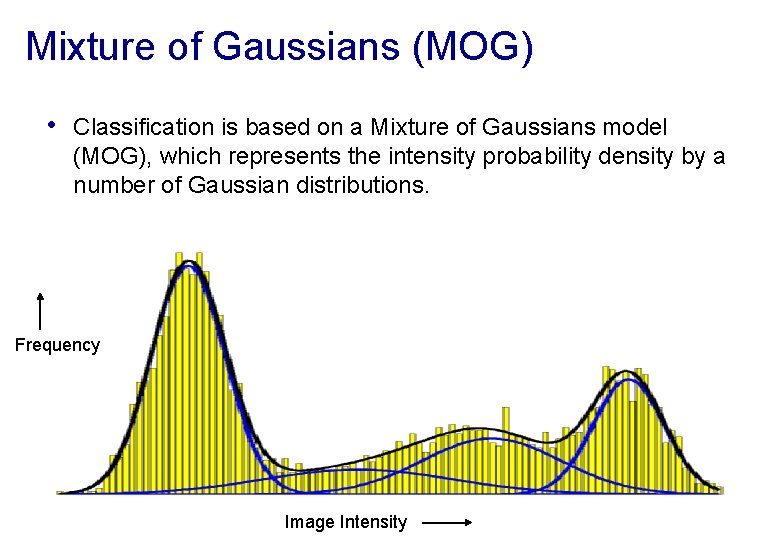
Mixture of Gaussians (MOG) • Classification is based on a Mixture of Gaussians model (MOG), which represents the intensity probability density by a number of Gaussian distributions. Frequency Image Intensity

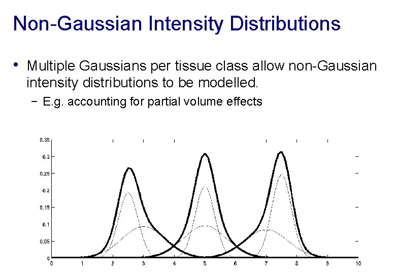
Non-Gaussian Intensity Distributions • Multiple Gaussians per tissue class allow non-Gaussian intensity distributions to be modelled. − E. g. accounting for partial volume effects

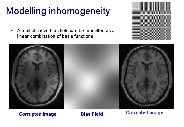
Modelling inhomogeneity • A multiplicative bias field can be modelled as a linear combination of basis functions. Corrupted image Bias Field Corrected image

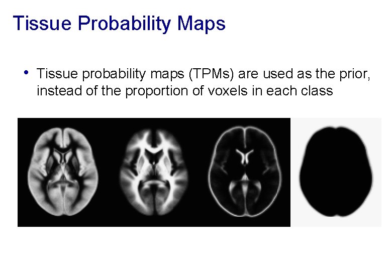
Tissue Probability Maps • Tissue probability maps (TPMs) are used as the prior, instead of the proportion of voxels in each class

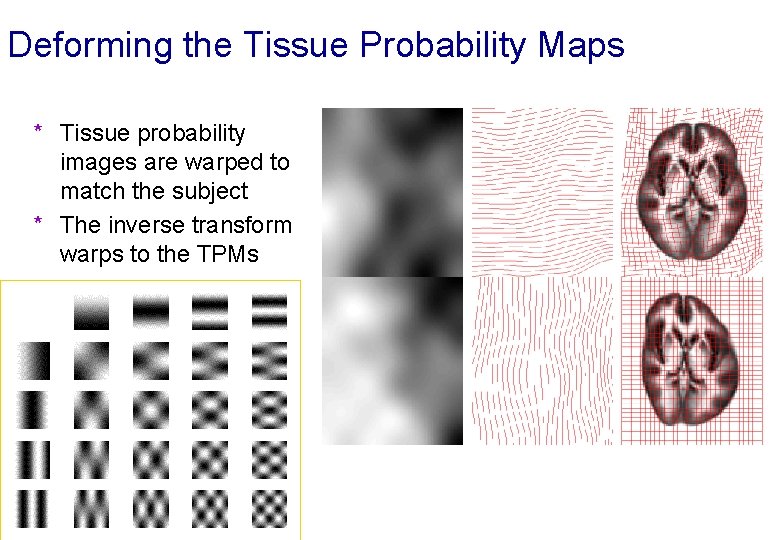
Deforming the Tissue Probability Maps * Tissue probability images are warped to match the subject * The inverse transform warps to the TPMs

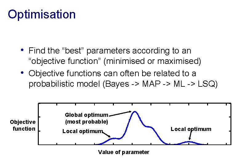
Optimisation • Find the “best” parameters according to an • “objective function” (minimised or maximised) Objective functions can often be related to a probabilistic model (Bayes -> MAP -> ML -> LSQ) Objective function Global optimum (most probable) Local optimum Value of parameter Local optimum

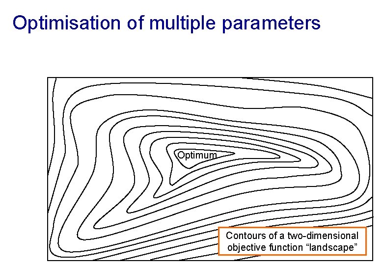
Optimisation of multiple parameters Optimum Contours of a two-dimensional objective function “landscape”

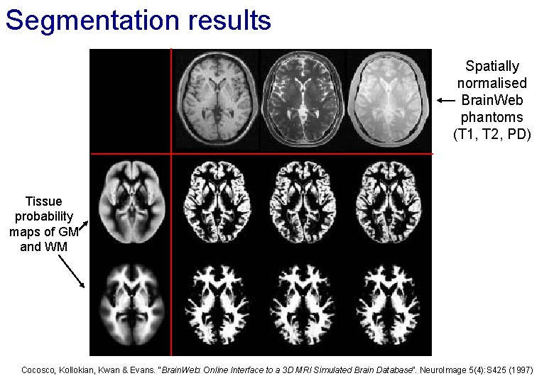
Segmentation results Spatially normalised Brain. Web phantoms (T 1, T 2, PD) Tissue probability maps of GM and WM Cocosco, Kollokian, Kwan & Evans. “Brain. Web: Online Interface to a 3 D MRI Simulated Brain Database”. Neuro. Image 5(4): S 425 (1997)

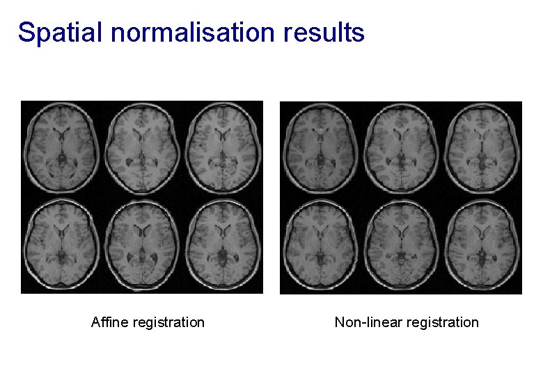
Spatial normalisation results Affine registration Non-linear registration

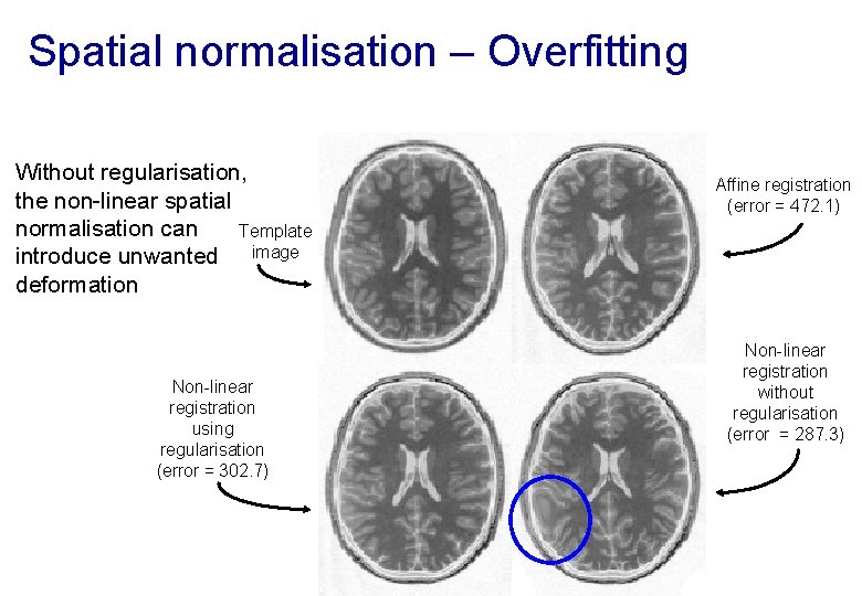
Spatial normalisation – Overfitting Without regularisation, the non-linear spatial normalisation can Template introduce unwanted image deformation Non-linear registration using regularisation (error = 302. 7) Affine registration (error = 472. 1) Non-linear registration without regularisation (error = 287. 3)

Spatial normalisation – regularisation • The “best” parameters according to the objective • function may not be realistic In addition to similarity, regularisation terms or constraints are often needed to ensure a reasonable solution is found − Also helps avoid poor local optima − Can be considered as priors in a Bayesian framework, e. g. converting ML to MAP: • log(posterior) = log(likelihood) + log(prior) + c

Spatial normalisation – Limitations • Seek to match functionally homologous regions, but. . . − − Challenging high-dimensional optimisation, many local optima Different cortices can have different folding patterns No exact match between structure and function [Interesting recent paper Amiez et al. (2013), PMID: 23365257 ] • Compromise − Correct relatively large-scale variability (sizes of structures) − Smooth over finer-scale residual differences

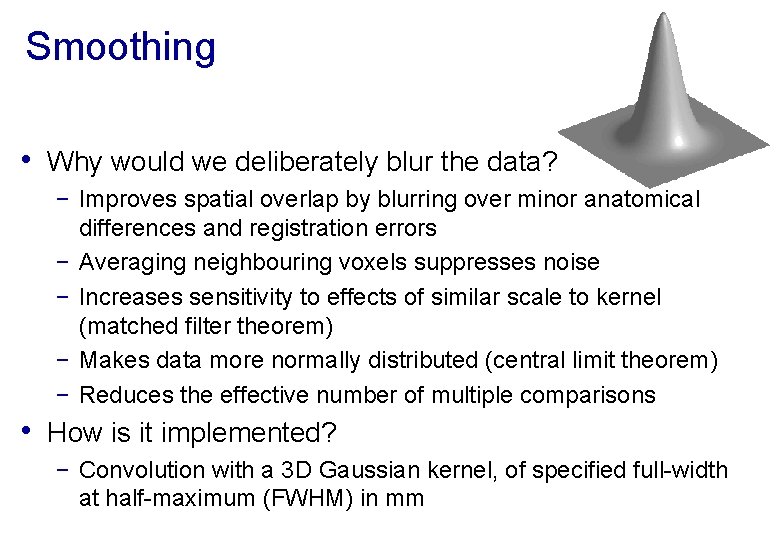
Smoothing • Why would we deliberately blur the data? − Improves spatial overlap by blurring over minor anatomical differences and registration errors − Averaging neighbouring voxels suppresses noise − Increases sensitivity to effects of similar scale to kernel (matched filter theorem) − Makes data more normally distributed (central limit theorem) − Reduces the effective number of multiple comparisons • How is it implemented? − Convolution with a 3 D Gaussian kernel, of specified full-width at half-maximum (FWHM) in mm

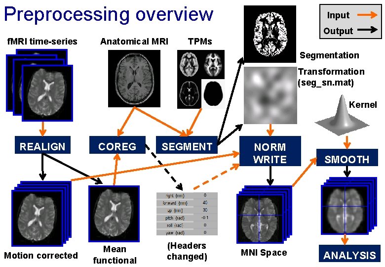
Preprocessing overview Input Output f. MRI time-series Anatomical MRI TPMs Segmentation Transformation (seg_sn. mat) Kernel REALIGN Motion corrected COREG Mean functional SEGMENT (Headers changed) NORM WRITE MNI Space SMOOTH ANALYSIS

References • Friston et al. Spatial registration and normalisation of images. • • Human Brain Mapping 3: 165 -189 (1995). Collignon et al. Automated multi-modality image registration based on information theory. IPMI’ 95 pp 263 -274 (1995). Ashburner et al. Incorporating prior knowledge into image registration. Neuro. Image 6: 344 -352 (1997). Ashburner & Friston. Nonlinear spatial normalisation using basis functions. Human Brain Mapping 7: 254 -266 (1999). Thévenaz et al. Interpolation revisited. IEEE Trans. Med. Imaging 19: 739 -758 (2000). Andersson et al. Modeling geometric deformations in EPI time series. Neuroimage 13: 903 -919 (2001). Ashburner & Friston. Unified Segmentation. Neuro. Image 26: 839 -851 (2005). Ashburner. A Fast Diffeomorphic Image Registration Algorithm. Neuro. Image 38: 95 -113 (2007). • See also Lars Kasper’s Zurich slides & Phys. IO Toolbox http: //www. translationalneuromodeling. org/spmcourse/

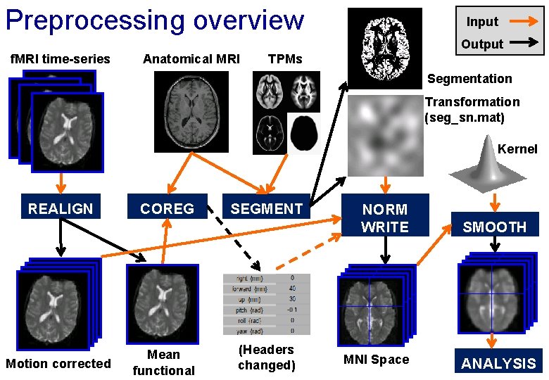
Preprocessing overview Input Output f. MRI time-series Anatomical MRI TPMs Segmentation Transformation (seg_sn. mat) Kernel REALIGN Motion corrected COREG Mean functional SEGMENT (Headers changed) NORM WRITE MNI Space SMOOTH ANALYSIS

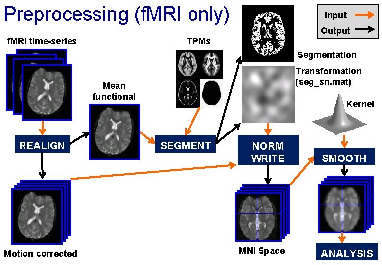
Preprocessing (f. MRI only) Input Output f. MRI time-series TPMs Segmentation Transformation (seg_sn. mat) Mean functional REALIGN Motion corrected Kernel SEGMENT NORM WRITE MNI Space SMOOTH ANALYSIS

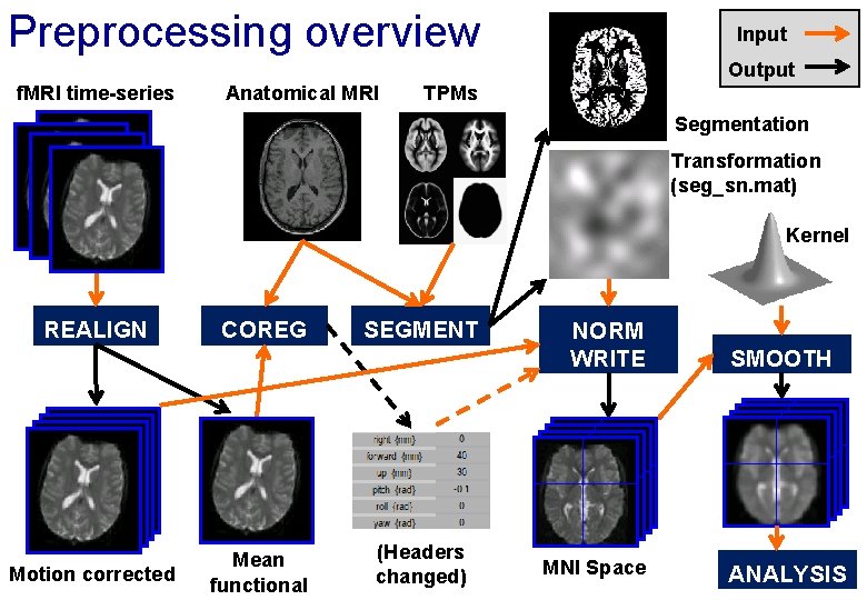
Preprocessing overview Input Output f. MRI time-series Anatomical MRI TPMs Segmentation Transformation (seg_sn. mat) Kernel REALIGN Motion corrected COREG Mean functional SEGMENT (Headers changed) NORM WRITE MNI Space SMOOTH ANALYSIS

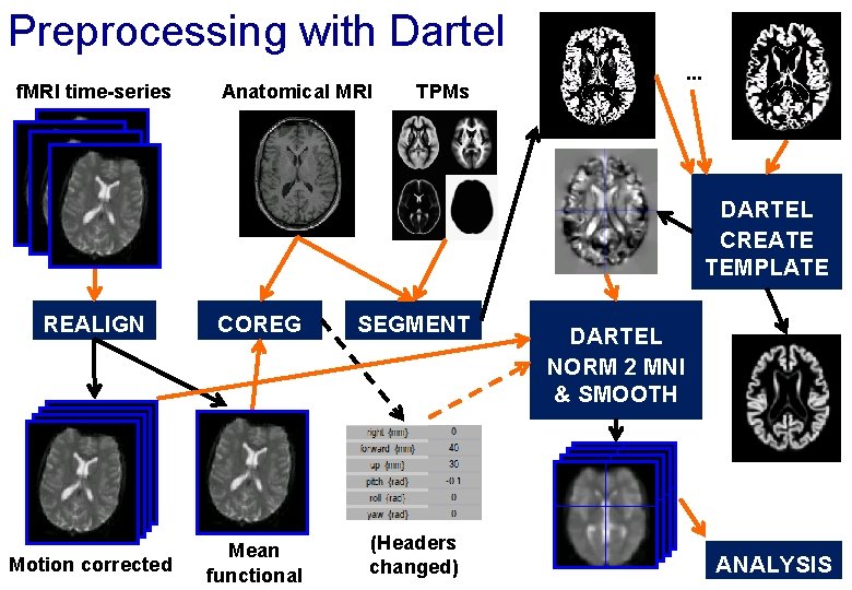
Preprocessing with Dartel f. MRI time-series Anatomical MRI . . . TPMs DARTEL CREATE TEMPLATE REALIGN COREG SEGMENT Motion corrected Mean functional (Headers changed) DARTEL NORM 2 MNI & SMOOTH ANALYSIS