Spatial Networks Outline 1 2 3 4 5

Spatial Networks

Outline 1. 2. 3. 4. 5. 6. 7. 8. 9. Motivation, and use cases Example spatial networks Conceptual model Need for SQL extensions CONNECT statement RECURSIVE statement Storage and data structures Algorithms for connectivity query Algorithms for shortest path

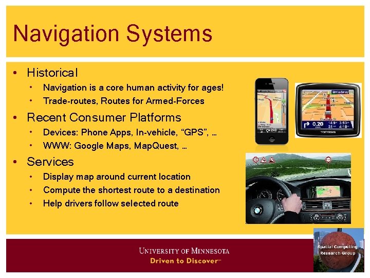
Navigation Systems • Historical • • Navigation is a core human activity for ages! Trade-routes, Routes for Armed-Forces • Recent Consumer Platforms • • Devices: Phone Apps, In-vehicle, “GPS”, … WWW: Google Maps, Map. Quest, … • Services • • • Display map around current location Compute the shortest route to a destination Help drivers follow selected route

Location Based Services • Location: Where am I ? – Geo-code: Place Name (or Street Address) <latitude, longitude> – Reverse Geo-code: <latitude, longitude> Place Name • Directory: What is around me? – Where is the nearest Clinic? Restaurant? Taxi? – List all Banks within 1 mile. • Routes: How do I get there? – What is the shortest path to get there? – …

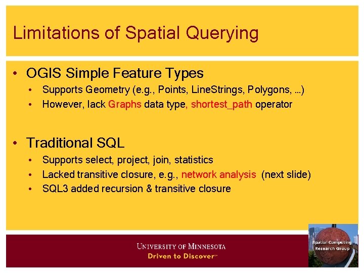
Limitations of Spatial Querying • OGIS Simple Feature Types • Supports Geometry (e. g. , Points, Line. Strings, Polygons, …) • However, lack Graphs data type, shortest_path operator • Traditional SQL • Supports select, project, join, statistics • Lacked transitive closure, e. g. , network analysis (next slide) • SQL 3 added recursion & transitive closure

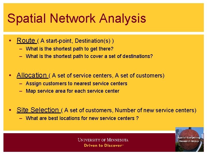
Spatial Network Analysis • Route ( A start-point, Destination(s) ) – What is the shortest path to get there? – What is the shortest path to cover a set of destinations? • Allocation ( A set of service centers, A set of customers) – Assign customers to nearest service centers – Map service area for each service center • Site Selection ( A set of customers, Number of new service centers) – What are best locations for new service centers ?

Outline 1. 2. 3. 4. 5. 6. 7. 8. 9. Motivation, and use cases Example spatial networks Conceptual model Need for SQL extensions CONNECT statement RECURSIVE statement Storage and data structures Algorithms for connectivity query Algorithms for shortest path

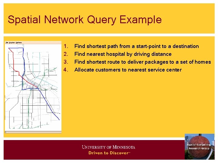
Spatial Network Query Example 1. 2. 3. 4. Find shortest path from a start-point to a destination Find nearest hospital by driving distance Find shortest route to deliver packages to a set of homes Allocate customers to nearest service center

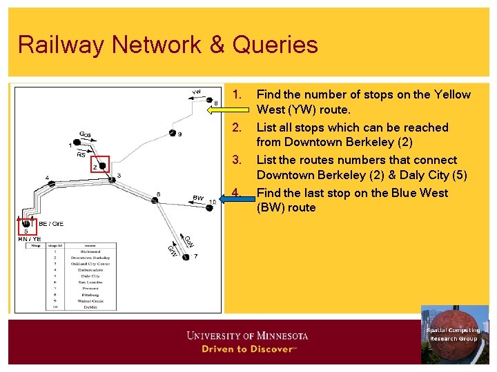
Railway Network & Queries 1. 2. 3. 4. Find the number of stops on the Yellow West (YW) route. List all stops which can be reached from Downtown Berkeley (2) List the routes numbers that connect Downtown Berkeley (2) & Daly City (5) Find the last stop on the Blue West (BW) route

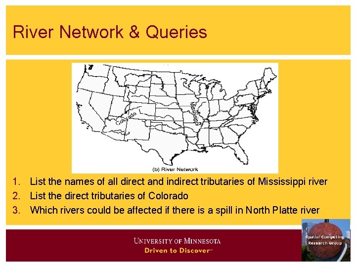
River Network & Queries 1. List the names of all direct and indirect tributaries of Mississippi river 2. List the direct tributaries of Colorado 3. Which rivers could be affected if there is a spill in North Platte river

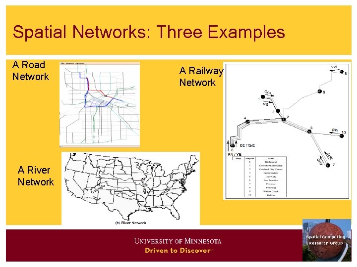
Spatial Networks: Three Examples A Road Network A River Network A Railway Network

Outline 1. 2. 3. 4. 5. 6. 7. 8. 9. Motivation, and use cases Example spatial networks Conceptual model Need for SQL extensions CONNECT statement RECURSIVE statement Storage and data structures Algorithms for connectivity query Algorithms for shortest path

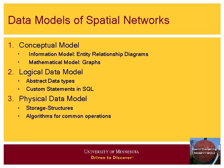
Data Models of Spatial Networks 1. Conceptual Model • • Information Model: Entity Relationship Diagrams Mathematical Model: Graphs 2. Logical Data Model • • Abstract Data types Custom Statements in SQL 3. Physical Data Model • • Storage-Structures Algorithms for common operations

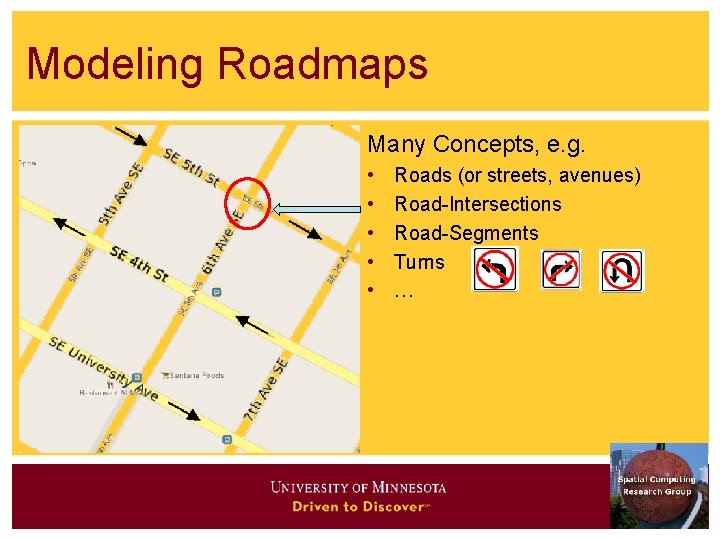
Modeling Roadmaps Many Concepts, e. g. • • • Roads (or streets, avenues) Road-Intersections Road-Segments Turns …

An Entity Relationship Diagram

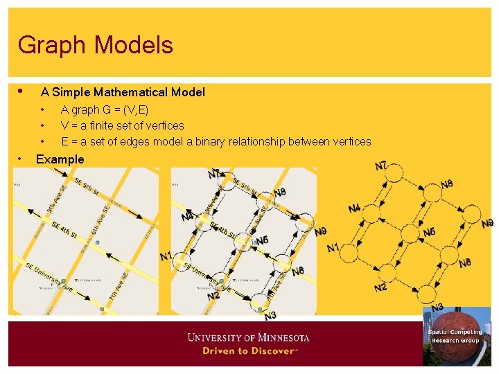
Graph Models • A Simple Mathematical Model • • A graph G = (V, E) V = a finite set of vertices E = a set of edges model a binary relationship between vertices Example

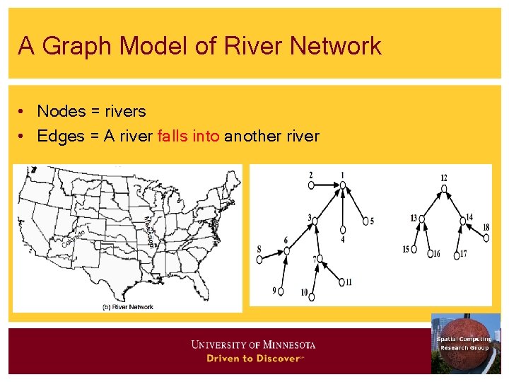
A Graph Model of River Network • Nodes = rivers • Edges = A river falls into another river

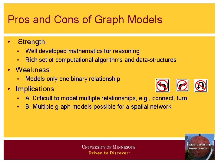
Pros and Cons of Graph Models • Strength • Well developed mathematics for reasoning • Rich set of computational algorithms and data-structures • Weakness • Models only one binary relationship • Implications • A. Difficult to model multiple relationships, e. g. , connect, turn • B. Multiple graph models possible for a spatial network

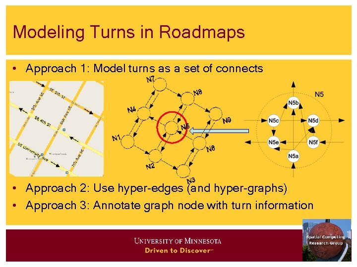
Modeling Turns in Roadmaps • Approach 1: Model turns as a set of connects • Approach 2: Use hyper-edges (and hyper-graphs) • Approach 3: Annotate graph node with turn information

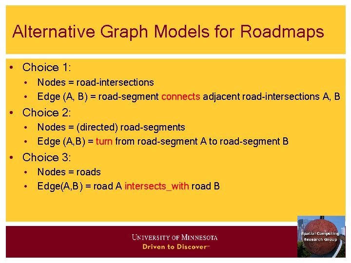
Alternative Graph Models for Roadmaps • Choice 1: • Nodes = road-intersections • Edge (A, B) = road-segment connects adjacent road-intersections A, B • Choice 2: • Nodes = (directed) road-segments • Edge (A, B) = turn from road-segment A to road-segment B • Choice 3: • Nodes = roads • Edge(A, B) = road A intersects_with road B

Quiz Which of the following are usually not captured in common graph models of roadmaps? a) Turn restrictions (e. g. , no U turn) b) Road intersections c) Road segments d) All of the above

Outline 1. 2. 3. 4. 5. 6. 7. 8. 9. Motivation, and use cases Example spatial networks Conceptual model Need for SQL extensions CONNECT statement RECURSIVE statement Storage and data structures Algorithms for connectivity query Algorithms for shortest path

Data Models of Spatial Networks 1. Conceptual Model: Entity Relationship Diagrams, Graphs 2. Logical Data Model & Query Languages • • Abstract Data types Custom Statements in SQL 3. Physical Data Model: Storage-Structures, Algorithms

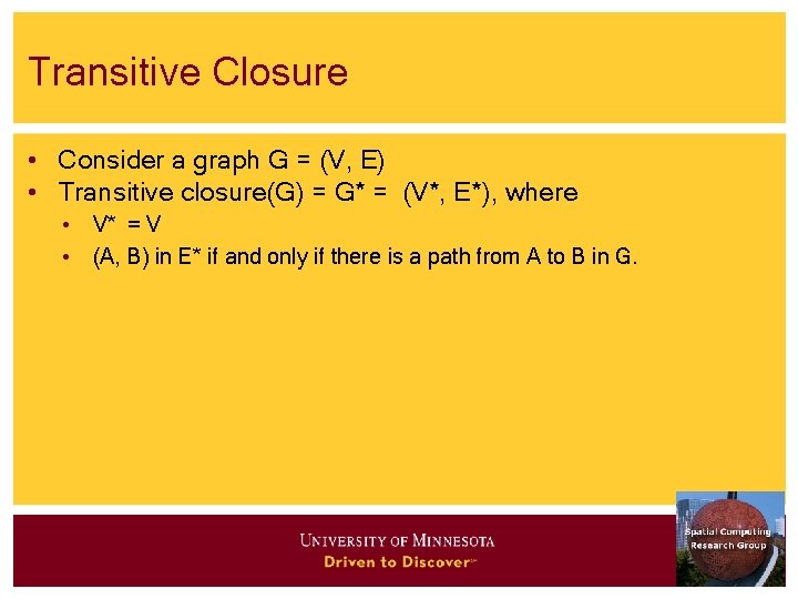
Transitive Closure • Consider a graph G = (V, E) • Transitive closure(G) = G* = (V*, E*), where • V* = V • (A, B) in E* if and only if there is a path from A to B in G.

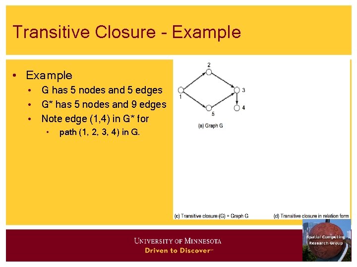
Transitive Closure - Example • G has 5 nodes and 5 edges • G* has 5 nodes and 9 edges • Note edge (1, 4) in G* for • path (1, 2, 3, 4) in G.

Limitations of Original SQL • Recall Relation algebra based languages • Ex. Original SQL • Can not compute transitive closure, e. g. , shortest path!

Supporting Graphs in SQL • Abstract Data Type (user defined) • SQL 3 • May include shortest path operation! • Custom Statements • SQL 2 - CONNECT clause in SELECT statement • For directed acyclic graphs, e. g. hierarchies • SQL 3 - WITH RECURSIVE statement • Transitive closure on general graphs

Outline 1. 2. 3. 4. 5. 6. 7. 8. 9. Motivation, and use cases Example spatial networks Conceptual model Need for SQL extensions CONNECT statement RECURSIVE statement Storage and data structures Algorithms for connectivity query Algorithms for shortest path

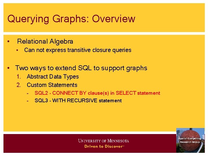
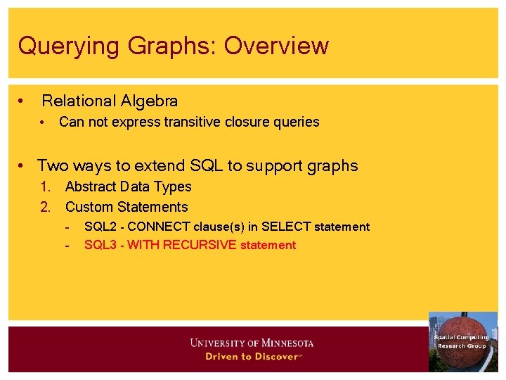
Querying Graphs: Overview • Relational Algebra • Can not express transitive closure queries • Two ways to extend SQL to support graphs 1. Abstract Data Types 2. Custom Statements – – SQL 2 - CONNECT BY clause(s) in SELECT statement SQL 3 - WITH RECURSIVE statement

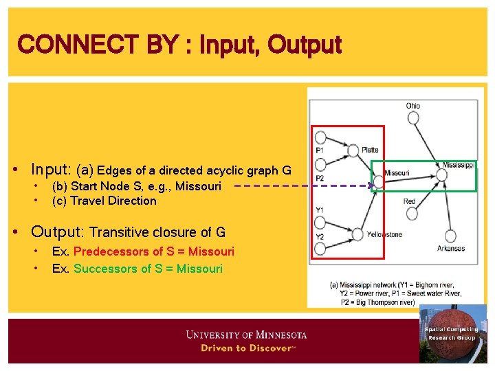
CONNECT BY : Input, Output • Input: (a) Edges of a directed acyclic graph G • • (b) Start Node S, e. g. , Missouri (c) Travel Direction • Output: Transitive closure of G • • Ex. Predecessors of S = Missouri Ex. Successors of S = Missouri

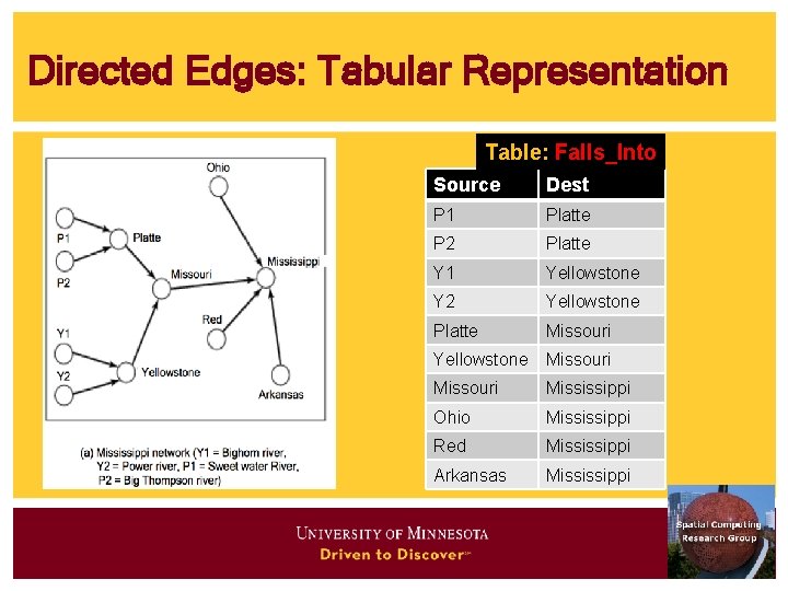
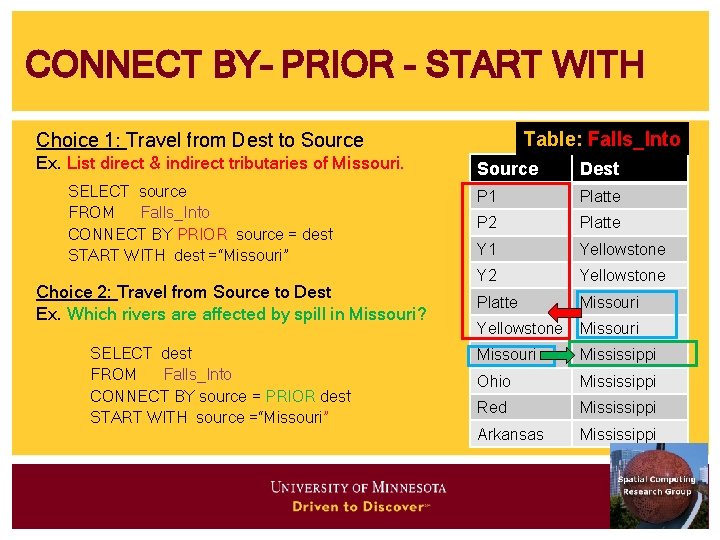
Directed Edges: Tabular Representation Table: Falls_Into Source Dest P 1 Platte P 2 Platte Y 1 Yellowstone Y 2 Yellowstone Platte Missouri Yellowstone Missouri Mississippi Ohio Mississippi Red Mississippi Arkansas Mississippi

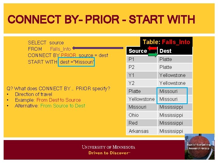
CONNECT BY– PRIOR - START WITH SELECT source FROM Falls_Into CONNECT BY PRIOR source = dest START WITH dest =“Missouri” Q? What does CONNECT BY … PRIOR specify? • Direction of travel • Example: From Dest to Source • Alternative: From Source to Dest Table: Falls_Into Source Dest P 1 Platte P 2 Platte Y 1 Yellowstone Y 2 Yellowstone Platte Missouri Yellowstone Missouri Mississippi Ohio Mississippi Red Mississippi Arkansas Mississippi

CONNECT BY– PRIOR - START WITH Table: Falls_Into Choice 1: Travel from Dest to Source Ex. List direct & indirect tributaries of Missouri. SELECT source FROM Falls_Into CONNECT BY PRIOR source = dest START WITH dest =“Missouri” Choice 2: Travel from Source to Dest Ex. Which rivers are affected by spill in Missouri? SELECT dest FROM Falls_Into CONNECT BY source = PRIOR dest START WITH source =“Missouri” Source Dest P 1 Platte P 2 Platte Y 1 Yellowstone Y 2 Yellowstone Platte Missouri Yellowstone Missouri Mississippi Ohio Mississippi Red Mississippi Arkansas Mississippi

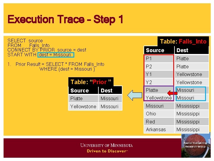
Execution Trace – Step 1 SELECT source FROM Falls_Into CONNECT BY PRIOR source = dest START WITH dest = Missouri Table: Falls_Into Source Dest P 1 Platte P 2 Platte Y 1 Yellowstone Table: “Prior ” Y 2 Yellowstone Source Dest Platte Missouri Yellowstone Missouri Mississippi Ohio Mississippi Red Mississippi Arkansas Mississippi 1. Prior Result = SELECT * FROM Falls_Into WHERE (dest = Missouri ) Yellowstone Missouri

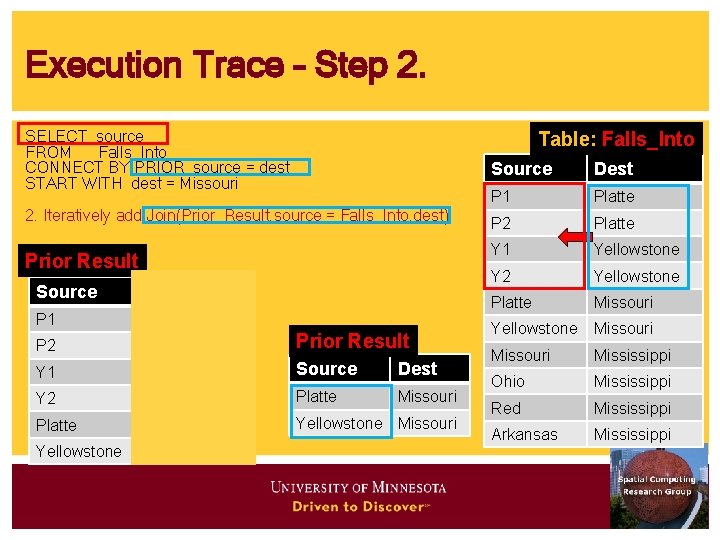
Execution Trace – Step 2. SELECT source FROM Falls_Into CONNECT BY PRIOR source = dest START WITH dest = Missouri Table: Falls_Into 2. Iteratively add Join(Prior_Result. source = Falls_Into. dest) Prior Result Source Dest P 1 Platte P 2 Platte Prior Result Y 1 Yellowstone Source Dest Y 2 Yellowstone Platte Missouri Yellowstone Missouri Source Dest P 1 Platte P 2 Platte Y 1 Yellowstone Y 2 Yellowstone Platte Missouri Yellowstone Missouri Mississippi Ohio Mississippi Red Mississippi Arkansas Mississippi

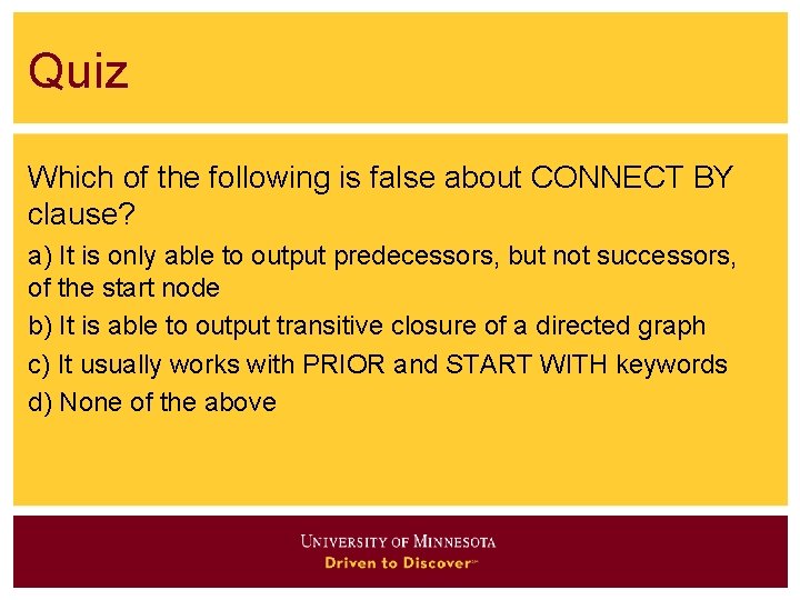
Quiz Which of the following is false about CONNECT BY clause? a) It is only able to output predecessors, but not successors, of the start node b) It is able to output transitive closure of a directed graph c) It usually works with PRIOR and START WITH keywords d) None of the above

Outline 1. 2. 3. 4. 5. 6. 7. 8. 9. Motivation, and use cases Example spatial networks Conceptual model Need for SQL extensions CONNECT statement RECURSIVE statement Storage and data structures Algorithms for connectivity query Algorithms for shortest path

Querying Graphs: Overview • Relational Algebra • Can not express transitive closure queries • Two ways to extend SQL to support graphs 1. Abstract Data Types 2. Custom Statements – – SQL 2 - CONNECT clause(s) in SELECT statement SQL 3 - WITH RECURSIVE statement

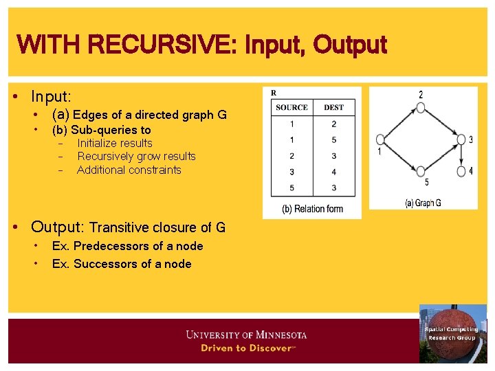
WITH RECURSIVE: Input, Output • Input: • (a) Edges of a directed graph G • (b) Sub-queries to – – – Initialize results Recursively grow results Additional constraints • Output: Transitive closure of G • • Ex. Predecessors of a node Ex. Successors of a node

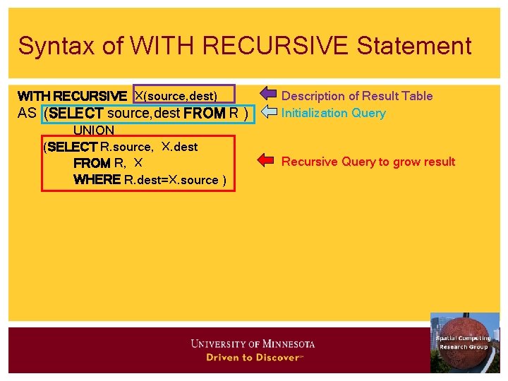
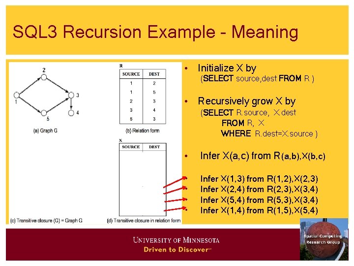
Syntax of WITH RECURSIVE Statement WITH RECURSIVE X(source, dest) AS (SELECT source, dest FROM R ) UNION (SELECT R. source, X. dest FROM R, X WHERE R. dest=X. source ) Description of Result Table Initialization Query Recursive Query to grow result

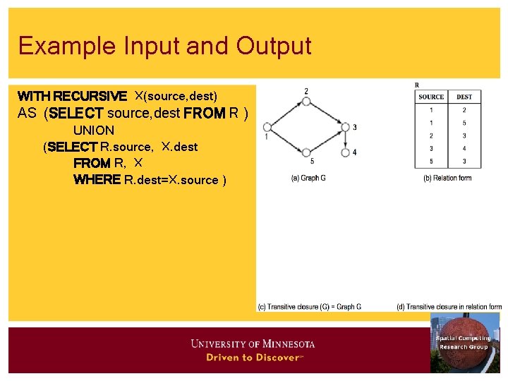
Example Input and Output WITH RECURSIVE X(source, dest) AS (SELECT source, dest FROM R ) UNION (SELECT R. source, X. dest FROM R, X WHERE R. dest=X. source )

SQL 3 Recursion Example - Meaning • Initialize X by (SELECT source, dest FROM R ) • Recursively grow X by (SELECT R. source, X. dest FROM R, X WHERE R. dest=X. source ) • Infer X(a, c) from R(a, b), X(b, c) • • Infer X(1, 3) from R(1, 2), X(2, 3) Infer X(2, 4) from R(2, 3), X(3, 4) Infer X(5, 4) from R(5, 3), X(3, 4) Infer X(1, 4) from R(1, 5), X(5, 4)

Quiz Which of the following are true about WITH RECURSIVE clause? a) It is able to output transitive closure of a directed graph b) It usually works with an edge table c) It includes two SELECT statements d) All of the above

Outline 1. 2. 3. 4. 5. 6. 7. 8. 9. Where do we use spatial networks? Example spatial networks Conceptual model of spatial networks Why do we need SQL extensions CONNECT clause RECURSIVE statement Data structures Algorithms for connectivity query Algorithms for shortest path

Data Models of Spatial Networks 1. Conceptual Model : Entity Relationship Diagrams, Graphs 2. Logical Data Model : Abstract Data types , Custom Statements in SQL 3. Physical Data Model • • Storage: Data-Structures, File-Structures Algorithms for common operations

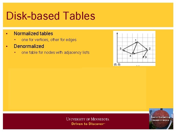
Main Memory Data-Structures • Adjacency matrix • • M[A, B] = 1 if and only if edge(vertex A, vertex B) exists Adjacency list : • maps a vertex to a list of its successors

Disk-based Tables • Normalized tables • • one for vertices, other for edges Denormalized • one table for nodes with adjacency lists

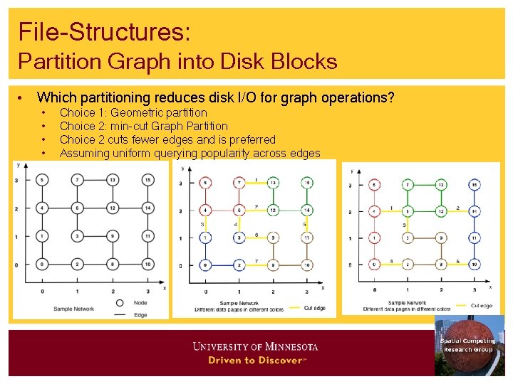
File-Structures: Partition Graph into Disk Blocks • Which partitioning reduces disk I/O for graph operations? • • Choice 1: Geometric partition Choice 2: min-cut Graph Partition Choice 2 cuts fewer edges and is preferred Assuming uniform querying popularity across edges

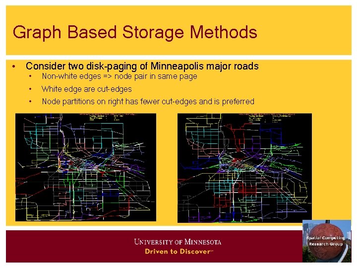
Graph Based Storage Methods • Consider two disk-paging of Minneapolis major roads • Non-white edges => node pair in same page • White edge are cut-edges • Node partitions on right has fewer cut-edges and is preferred

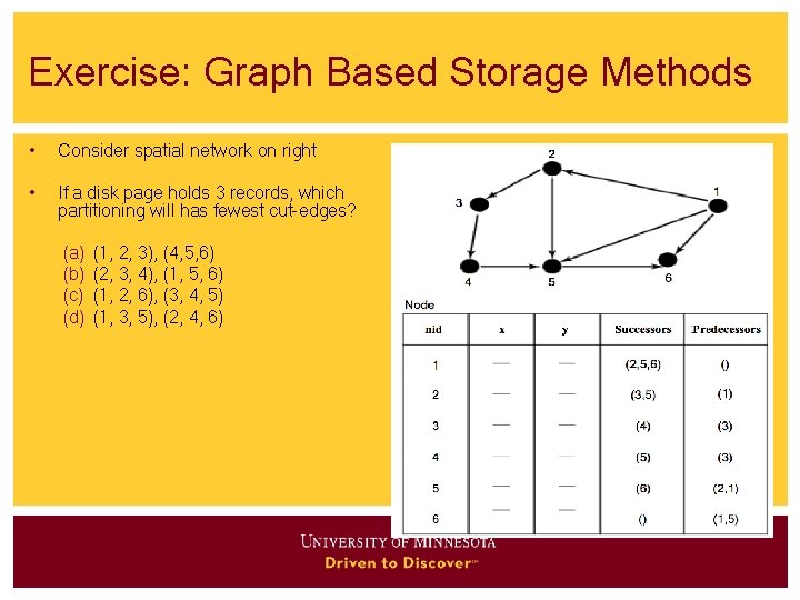
Exercise: Graph Based Storage Methods • Consider spatial network on right • If a disk page holds 3 records, which partitioning will has fewest cut-edges? (a) (b) (c) (d) (1, 2, 3), (4, 5, 6) (2, 3, 4), (1, 5, 6) (1, 2, 6), (3, 4, 5) (1, 3, 5), (2, 4, 6)

Outline 1. 2. 3. 4. 5. 6. 7. 8. 9. Motivation, and use cases Example spatial networks Conceptual model Need for SQL extensions CONNECT statement RECURSIVE statement Storage and data structures Algorithms for connectivity query Algorithms for shortest path

Data Models of Spatial Networks 1. Conceptual Model : Entity Relationship Diagrams, Graphs 2. Logical Data Model : Abstract Data types , Custom Statements in SQL 3. Physical Data Model • • Storage-Structures Algorithms for common operations

Query Processing for Spatial Networks • Query Processing • • • DBMS decomposes a query into building blocks Keeps a couple of strategy for each building block Selects most suitable one for a given situation • Building blocks • Connectivity(A, B): Is node B reachable from node A? • Shortest path(A, B): Identify least cost path from node A to node B

Algorithms • Main memory • • • Connectivity: Breadth first search, depth first search Shortest path: Dijkstra’s algorithm, A* Disk-based • • Shortest path - Hierarchical routing algorithm Connectivity strategies are in SQL 3

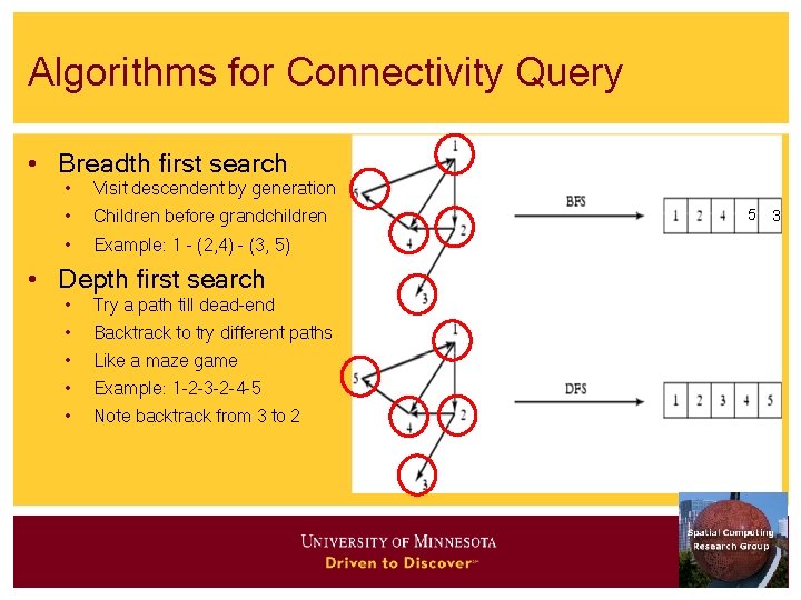
Algorithms for Connectivity Query • Breadth first search • Visit descendent by generation • Children before grandchildren • Example: 1 - (2, 4) - (3, 5) • Depth first search • Try a path till dead-end • Backtrack to try different paths • Like a maze game • Example: 1 -2 -3 -2 -4 -5 • Note backtrack from 3 to 2 5 3

Outline 1. 2. 3. 4. 5. 6. 7. 8. 9. Motivation, and use cases Example spatial networks Conceptual model Need for SQL extensions CONNECT statement RECURSIVE statement Storage and data structures Algorithms for connectivity query Algorithms for shortest path

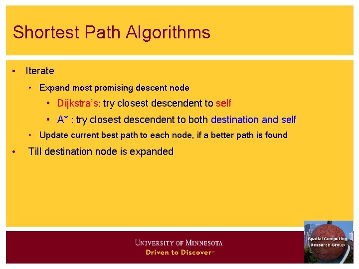
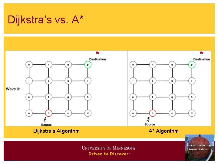
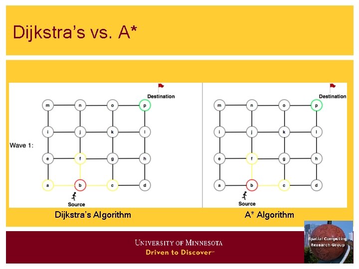
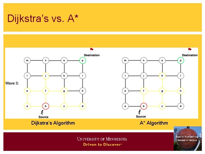
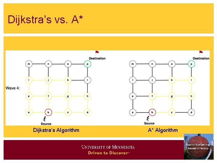
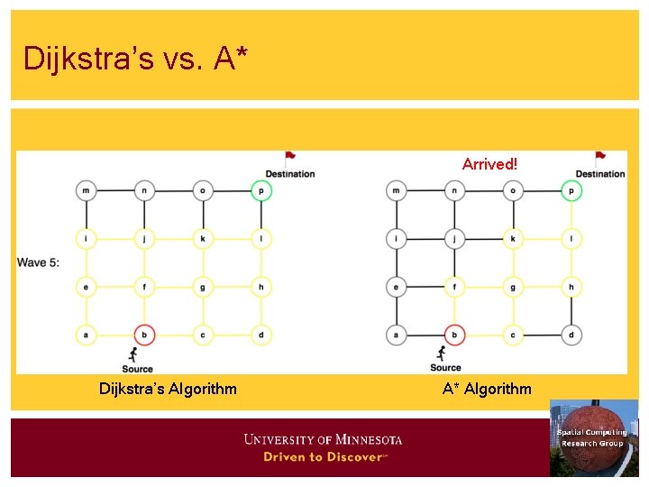
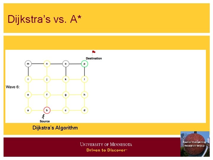
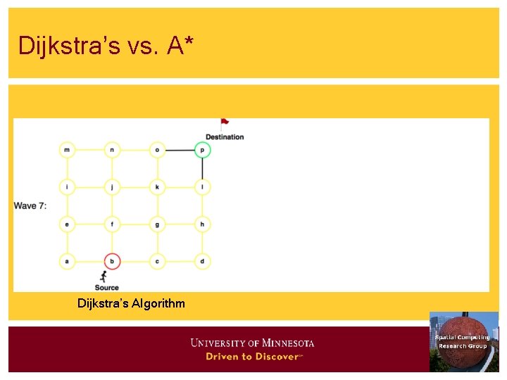
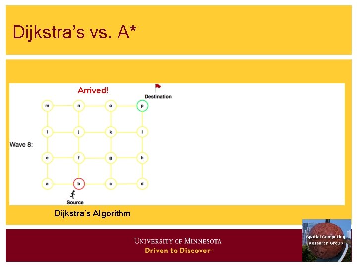
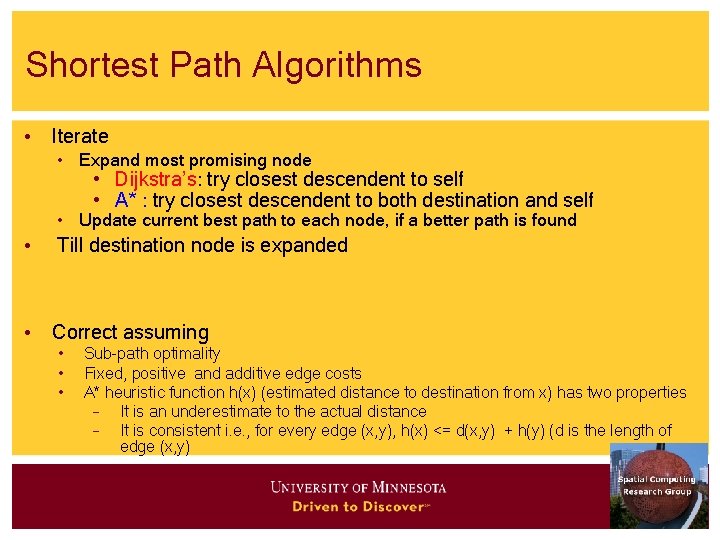
Shortest Path Algorithms • Iterate • Expand most promising descent node • Dijkstra’s: try closest descendent to self • A* : try closest descendent to both destination and self • Update current best path to each node, if a better path is found • Till destination node is expanded

Dijkstra’s vs. A* Dijkstra’s Algorithm A* Algorithm

Dijkstra’s vs. A* Dijkstra’s Algorithm A* Algorithm

Dijkstra’s vs. A* Dijkstra’s Algorithm A* Algorithm

Dijkstra’s vs. A* Dijkstra’s Algorithm A* Algorithm

Dijkstra’s vs. A* Dijkstra’s Algorithm A* Algorithm

Dijkstra’s vs. A* Arrived! Dijkstra’s Algorithm A* Algorithm

Dijkstra’s vs. A* Dijkstra’s Algorithm

Dijkstra’s vs. A* Dijkstra’s Algorithm

Dijkstra’s vs. A* Arrived! Dijkstra’s Algorithm

Shortest Path Algorithms • Iterate • Expand most promising node • Dijkstra’s: try closest descendent to self • A* : try closest descendent to both destination and self • Update current best path to each node, if a better path is found • Till destination node is expanded • Correct assuming • • • Sub-path optimality Fixed, positive and additive edge costs A* heuristic function h(x) (estimated distance to destination from x) has two properties – It is an underestimate to the actual distance – It is consistent i. e. , for every edge (x, y), h(x) <= d(x, y) + h(y) (d is the length of edge (x, y)

Shortest Path Strategies - 3 • Dijkstra’s and Best first algorithms • Work well when entire graph is loaded in main memory • Otherwise their performance degrades substantially • Hierarchical Routing Algorithms • Works with graphs on secondary storage • Loads small pieces of the graph in main memories • Can compute least cost routes

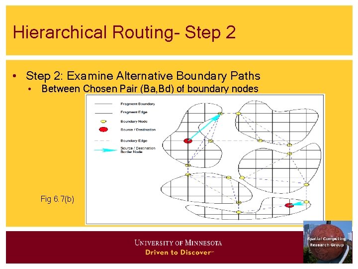
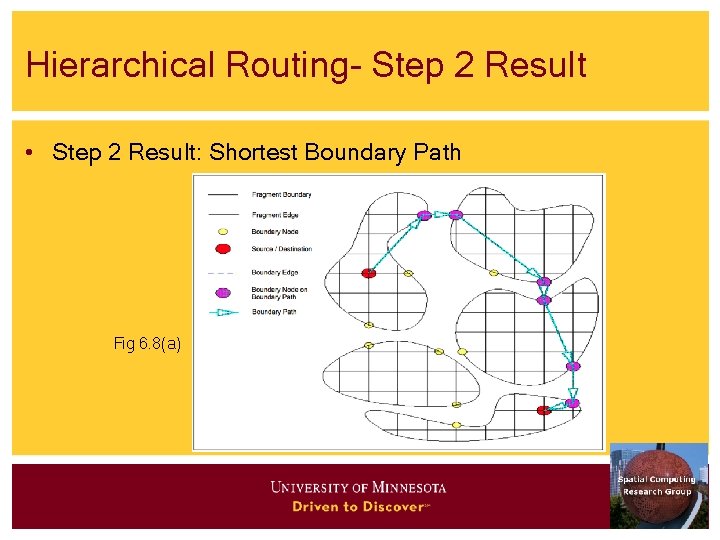
Shortest Path Strategies - 3 (Key Ideas) • Key ideas behind Hierarchical Routing Algorithm • Fragment graphs - pieces of original graph obtained via node partitioning • Boundary nodes - nodes of with edges to two fragments • Boundary graph - a summary of original graph • Contains Boundary nodes • Boundary edges: edges across fragments or paths within a fragment

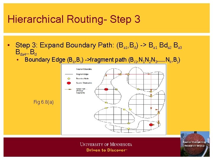
Shortest Path Strategies – 3 (Insight) • A Summary of Optimal path in original graph can be computed • Using Boundary graph and 2 fragments • The summary can be expanded into optimal path in original graph • Examining a fragments overlapping with the path • Loading one fragment in memory at a time

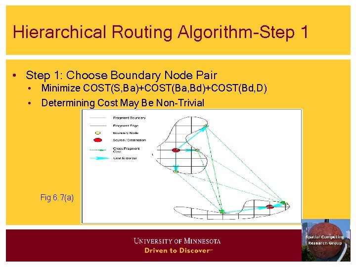
Shortest Path Strategies – 3 (Illustration of the Algorithm) • Figure 6. 7(a) - fragments of source and destination nodes • Figure 6. 7(b) - computing summary of optimal path using • Boundary graph and 2 fragments • Note use of boundary edges only in the path computation • Figure 6. 8(a) - The summary of optimal path using boundary edges • Figure 6. 8(b) Expansion back to optimal path in original graph

Hierarchical Routing Algorithm-Step 1 • Step 1: Choose Boundary Node Pair • Minimize COST(S, Ba)+COST(Ba, Bd)+COST(Bd, D) • Determining Cost May Be Non-Trivial Fig 6. 7(a)

Hierarchical Routing- Step 2 • Step 2: Examine Alternative Boundary Paths • Between Chosen Pair (Ba, Bd) of boundary nodes Fig 6. 7(b)

Hierarchical Routing- Step 2 Result • Step 2 Result: Shortest Boundary Path Fig 6. 8(a)

Hierarchical Routing- Step 3 • Step 3: Expand Boundary Path: (Ba 1, Bd) -> Ba 1 Bda 2 Ba 3 Bda 4…Bd • Boundary Edge (Bij, Bj) ->fragment path (Bi 1, N 1 N 2 N 3……. Nk, Bj) Fig 6. 8(a)

Quiz Which of the following is false? a) Hierarchical routing algorithms are Disk-based shortest path algorithms b) Breadth first search and depth first search are both connectivity query algorithms c) Best first algorithm is always faster than Dijkstra’s algorithm d) None of the above